Understanding Image Generation: A Beginner’s Guide to Generative Adversarial Networks

All the code related to this article is available in our dedicated GitHub repository. You can reproduce all the experiments with OVHcloud AI Notebooks.

Have you ever been amazed by what generative artificial intelligence could do, and wondered how it can generate realistic images 🤯🎨?

In this tutorial, we will embark on an exciting journey into the world of Generating Adversarial Networks (GANs), a revolutionary concept in generative AI. No prior experience is necessary to follow along. We will walk you through every step, starting with the basic concepts and gradually building up to the implementation of Deep Convolutional GANs (DCGANs).

By the end of this tutorial, you will be able to generate your own images!

Introduction

GANs have been introduced by Ian Goodfellow et al. in 2014 in the paper Generative Adversarial Nets. GANs have become very popular last years, allowing us, for example, to:

• Generate high-resolution images (avatars, objects and scenes)
• Augment our data (generating synthetic (fake) data samples for limited datasets)
• Enhance the resolution of low-resolution images (upscaling images)
• Transfer image style of one image to another (Black and white to color)
• Predict facial appearances at different ages (Face Aging)

What is a GAN and how it works?

A GAN is composed of two main components: a generator G and a discriminator D.

Each component is a neural network, but their roles are different:

• The purpose of the generator G is to reproduce the data distribution of the training data 𝑥, to generate synthetic samples for the same data distribution. These data are often images, but can also be audio or text.

• On the other hand, the discriminator D is a kind of judge who will estimate whether a sample 𝑥 is real or fake (has been generated). It is in fact a classifier that will say if a sample comes from the real data distribution or the generator.

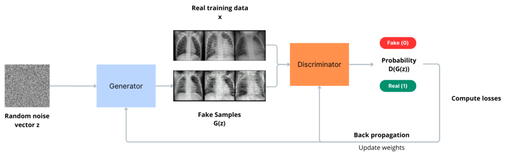
Illustration of GAN training

During training, the generator starts with a vector of random noise (z) as input and produces synthetic samples G(z).

As training progresses, it refines its output, making the generated data G(z) more and more similar to the real data. The goal of the generator is to outsmart the discriminator into classifying its generated samples as real.

Meanwhile, the discriminator is presented with both real samples from the training data and fake samples from the generator. As it learns to discriminate between the two, it provides feedback to the generator about the quality of its generated samples. This is why the term “adversarial“ is used here.

Mathematical approach

In fact, GANs come from game theory, where D and G are playing a two-player minimax game with the following value function:

As we can observe, the discriminator aims to maximize the V function. To do this, it must maximize each of the two parts of the equation that will be added together. This means maximizing log(D(x)), so D(x) in the first equation part (probability of real data), and minimizing the D(G(z)) in the second part (probability of fake data).

Simultaneously, the generator tries to minimize the function. It only comes into play in the second part of the function, where it tries to obtain the highest value of D(G(z)) in order to fool the discriminator.

This constant confrontation between the generator and the discriminator creates an iterative learning process, where the generator gradually improves to produce increasingly realistic G(z) samples, and the discriminator becomes increasingly accurate in its distinction of the data presented to it.

In an ideal scenario, this iterative process would reach an equilibrium point, where the generator produces data that is indistinguishable from real data, and the discriminator’s performance is 50% (random guessing).

GANs may not always reach this equilibrium due to the training process being sensitive to factors (architecture, hyperparameters, dataset complexity). The generator and discriminator may reach a dead end, oscillating between solutions or facing mode collapse, resulting in limited sample diversity. Also, it is important that discriminator does not start off too strong, otherwise the generator will not get any information on how to improve itself, since it does not know what the real data looks like, as shown in the illustration above.

DCGAN (Deep Convolutional GANs)

DCGAN has been introduced in 2016 by Alec Radford et al. in the paper Unsupervised Representation Learning with Deep Convolutional Generative Adversarial Networks.

Its new convolutional architecture has considerably improved the quality and stability of image synthesis compared to classical GANs. Here are the major changes:

• Replace any pooling layers with strided convolutions (discriminator) and fractional-strided convolutions (generator), making them exceptionally well-suited for image generation tasks.
• Use batchnorm in both the generator and the discriminator.
• Removing fully connected hidden layers for deeper architectures.
• Use ReLU activation in generator for all layers except for the output, which uses tanh.
• Use LeakyReLU activation in the discriminator for all layer.

The operation principles of these layers will not be explained in this tutorial.

Use case & Objective

Now that we know the concept of image generation, let’s try to put it into practice!

In this tutorial, we will implement a DCGAN architecture and train it on a medical dataset to generate new images. This dataset is the Chest X-Ray Pneumonia. All the code explained here will run on a single GPU, linked to OVHcloud AI Notebooks, and is given in our GitHub repository.

1 – Explore dataset and prepare it for training

The Chest X-Ray Pneumonia dataset contains 5,863 X-Ray images. This may not be sufficient for training a robust DCGAN, but we are going to try! Indeed, the DCGAN research paper is conducting its study on a dataset of over 60,000 images.

Additionally, it is important to consider that the dataset contains two classes (Pneumonia/Normal). While we will not separate the classes for data quantity purposes, improving our network’s performance could be beneficial. Furthermore, it is advisable to verify if the classes are well-balanced.

Only the training subset will be used here (5,221 images). Let’s take a look at our images:

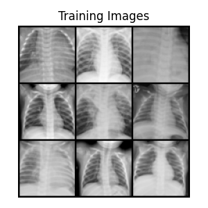
We notice that we have quite similar images. The backgrounds are identical, and the chests are often centered in the same way, which should help the network learn.

Preprocessing

Data pre-processing is a crucial step when you want to facilitate and accelerate model convergence and obtain high-quality results. This pre-processing can be broken down into various generic operations that are commonly applied.

Each image in the dataset will be transformed. They are then assembled in packets of 128 images, which we call batches. This avoids loading the dataset all at once, which could use up a lot of memory. This also makes the most of GPUs parallelism.

The applied transformation will:

• Resize images to (64x64xchannels), dimensions expected by our DCGAN. This avoids keeping the original dimensions of the images, which are all different. This also reduces the number of pixels which accelerates the model training (computation cost).
• Convert images to tensors (format expected by models).
• Standardize & Normalize the image’s pixel values, which improves training performance in AI.

If original images are smaller than the desired size, transformation will pad the images to reach the specified size.

We won’t show you the code for these transformations here, but as mentioned earlier, you can find it in its entirety on our GitHub repository. You can reproduce all the experiments with OVHcloud AI Notebooks.

Step 2 – Define the models

Now that the images are ready, we can define our DCGAN:

Generator implementation

As shown in the image above, the generator architecture is designed to take a random noise vector z as input and transform it into a (3x64x64) image, which is the same size as the images in the training dataset.

To do this, it uses transposed convolutions (also falsely known as deconvolutions) to progressively upsample the noise vector z until it reaches the desired output image size. In fact, the transposed convolutions help the generator capture complex patterns and generate realistic images during the training process.

The final Tanh() activation function ensures that the pixel values of the generated images are in the range [-1, 1], which also corresponds to our transformed training images (we had normalized them).

The code for implementing this generator is given in its entirety on our GitHub repository.

Discriminator implementation

As a reminder, the discriminator acts as a sample classifier. Its aim is to distinguish the data generated by the generator from the real data in the training dataset.

As shown in the image above, the discriminator takes an input image of size (3x64x64) and outputs a probability, indicating if the input image is real (1) or fake (0).

To do this, it uses convolutional layers, batch normalization layers, and LeakyReLU functions, which are presented in the paper as architecture guidelines to follow. Each convolutional block is designed to capture features of the input images, moving from low-level features such as edges and textures for the first blocks, to more abstract and complex features such as shapes and objects for the last.

Probability is obtained thanks to the use of the sigmoid activation, which squashes the output to the range [0, 1].

The code for implementing this discriminator is given in its entirety on our GitHub repository.

Define loss function and labels

Now that we have our adversarial networks, we need to define the loss function.

The adversarial loss V(D, G) can be approximated using the Binary Cross Entropy (BCE) loss function, which is commonly used for GANs because it measures the binary cross-entropy between the discriminator’s output (probability) and the ground truth labels during training (here we fix real=1 or fake=0). It will calculate the loss for both the generator and the discriminator during backpropagation.

BCE Loss is computed with the following equation, where target is the ground truth label (1 or 0), and ŷ is the discriminator’s probability output:

If we compare this equation to our previous V(D, G) objective, we can see that BCE loss term for real data samples corresponds to the first term in V(D, G), log(D(x)), and the BCE loss term for fake data samples corresponds to the second term in V(D, G), log(1 – D(G(z))).

In this binary case, the BCE can be represented by two distinct curves, which describe how the loss varies as a function of the predictions ŷ of the model. The first shows the loss as a function of the calculated probability, for a synthetic sample (label y = 0). The second describes the loss for a real sample (label y = 1).

We can see that the further the prediction ŷ is from the actual label assigned (target), the greater the loss. On the other hand, a prediction that is close to the truth will generate a loss very close to zero, which will not impact the model since it appears to classify the samples successfully.

During training, the goal is to minimize the BCE loss. This way, the discriminator will learn to correctly classify real and generated samples, while the generator will learn to generate samples that can “fool” the discriminator into classifying them as real.

Hyperparameters

Hyperparameters were chosen according to the indications given by in the DCGAN paper.

Step 3 – Train the model

We are now ready to train our DCGAN !

To monitor the generator’s learning progress, we will create a constant noise vector, denoted as fixed_noise.

During the training loop, we will regularly feed this fixed_noise into the generator. Using a same constant vector makes it possible to generate similar images each time, and to observe the evolution of the samples produced by the generator over the training cycles.

fixed_noise = torch.randn(64, nz, 1, 1, device=device)

Also, we will compute the BCE Loss of the Discriminator and the Generator separately. This will enable them to improve over the training cycles. For each batch, these losses will be calculated and saved into lists, enabling us to plot the losses after training for each training iteration.

Training Process

Thanks to our fixed noise vector, we were able to capture the evolution of the generated images, providing an overview of how the model learned to reproduce the distribution of training data over time.

Here are the samples generated by our model during training, when fed with a fixed noise, over 100 epochs. For visualization, a display of 9 generated images was chosen :

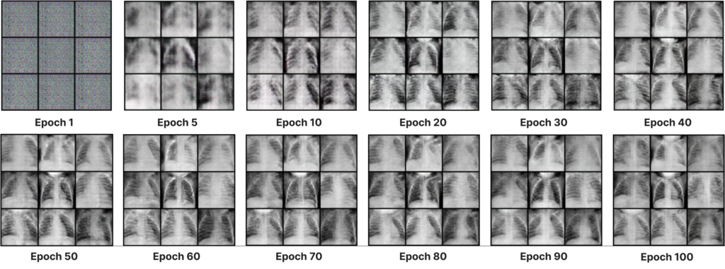
At the start of the training process (epoch 1), the images generated show the characteristics of the random noise vector.

As the training progresses, the weights of the discriminator and generator are updated. Noticeable changes occur in the generated images. Epochs 5, 10 and 20 show quick and subtle evolution of the model, which begins to capture more distinct shapes and structures.

Next epochs show an improvement in edges and details. Generated samples become sharper and more identifiable, and by epoch 100 the images are quite realistic despite the limited data available (5,221 images).

Do not hesitate to play with the hyperparameters to try and vary your results! You can also check out the GAN hacks repo, which shares many tips dedicated to training GANs. Training time will vary according to your resources and the number of images.

Step 4 – Results & Inference

Once the generator has been trained over 100 epochs, we are free to generated unlimited new images, based on a new random noise vector each time.

In order to retain only relevant samples, a data post-processing step was set up to assess the quality of the images generated. All generated images were sent to the trained discriminator. Its job is to evaluate the probability of the generated samples, and keep only those which have obtained a probability greater than a fixed threshold (0.8 for example).

This way, we have obtained the following images, compared to the original ones. We can see that despite the small number of images in our dataset, the model was able to identify and learn the distribution of the real images data and reproduce them in a realistic way:

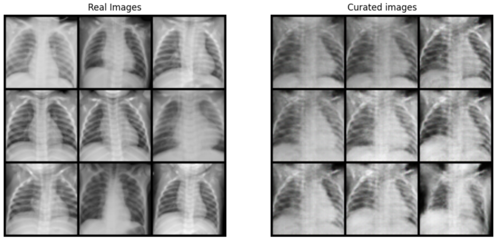
Original dataset images (left), compared with images selected from generated samples (right)

Step 5 – Evaluate the model

A DCGAN model (and GANs in general) can be evaluated in several ways. A research paper has been published on this subject.

Quantitative measures

On the quantitative side, the evolution of the BCE loss of the generator and the discriminator provide indications of the quality of the model during training.

The evolution of these losses is illustrated in the figure below, where the discriminator losses are shown in orange and the generator losses in blue, over a total of 4100 iterations. Each iteration corresponds to a complete pass of the dataset, which is split into 41 batches of 128 images. Since the model has been trained over 100 epochs, loss tracking is available over 4100 iterations (41*100).

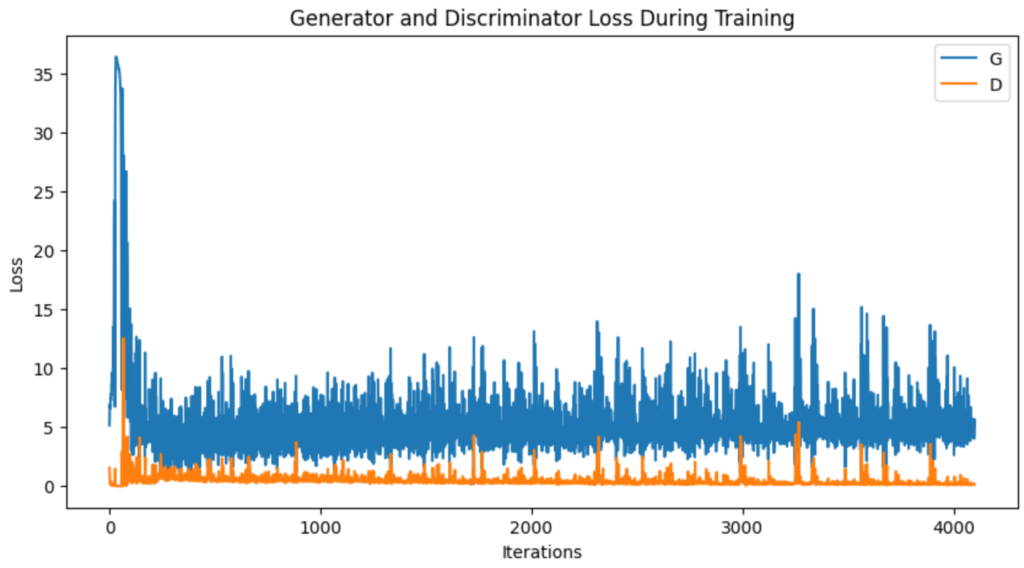
At the start of training, both curves show high loss values, indicating an unstable start of the DCGAN. This results in very unrealistic images being generated, where the nature of the random noise is still too present (see epoch 1 on the previous image). The discriminator is therefore too powerful for the moment.

A few iterations later, the losses converge towards lower values, demonstrating the improvement in the model’s performance.

However, from epoch 10, a trend emerges. The discriminator loss begins to decrease very slightly, indicating an improvement in its ability to determine which samples are genuine and which are synthetic. On the other hand, the generator’s loss shows a slight increase, suggesting that it needs to improve in order to generate images capable of deceiving its adversary.

More generally, fluctuations are observed throughout training due to the competitive nature of the network, where the generator and discriminator are constantly adjusting relative to each other. These moments of fluctuation may reflect attempts to adjust the two networks. Unfortunately, they do not ultimately appear to lead to an overall reduction in network loss.

Qualitative measures

Losses are not the only performance indicator. They are often insufficient to assess the visual quality of the images generated.

This is confirmed by an analysis of the previous graphs, where we inevitably notice that the images generated at epoch 10 are not the most realistic, while the loss is approximately the same as that obtained at epoch 100.

One commonly used method is human visual assessment. However, this manual assessment has a number of limitations. It is subjective, does not fully reflect the capabilities of the models, cannot be reproduced and is expensive.

Research is therefore focusing on finding new, more reliable and less costly methods. This is particularly the case with CAPTCHAs, tests designed to check whether a user is a human or a robot before accessing content. These tests sometimes present pairs of generated and real images where the user has to indicate which of the two seems more authentic. This ultimately amounts to training a discriminator and a generator manually.

All the code related to this article is available in our dedicated GitHub repository. You can reproduce all the experiments with OVHcloud AI Notebooks.

Conclusion

I hope you have enjoyed this post!

You are now more comfortable with image generation and the concept of Generative Adversarial Networks! Now you know how to generate images from your own dataset, even if it’s not very large!

You can train your own network on your dataset and generate images of faces, objects and landscapes. Happy GANning! 🎨🚀

You can check our other computer vision articles to learn how to:

• Perform Brain tumor segmentation using U-Net
• Train YOLOv5 on a custom dataset Object detection:

Paper references

• Generative Adversarial Nets, Ian Goodfellow, 2014
• Unsupervised Representation Learning with Deep Convolutional Generative Adversarial Networks, Alec Radford et al., 2016
• Pros and Cons of GAN Evaluation Measures, Ali Borji, 2018