Image segmentation: Train a U-Net model to segment brain tumors

A guide to discover image segmentation and train a convolutional neural network on medical images to segment brain tumors

All the code related to this article is available in our dedicated GitHub repository. You can reproduce all the experiments with AI Notebooks.

Over the past few years, the field of computer vision has experienced a significant growth. It encompasses a wide range of methods for acquiring, processing, analyzing and understanding digital images.

Among these methods, one is called image segmentation.

What is Image Segmentation? 🤔

Image segmentation is a technique used to separate an image into multiple segments or regions, each of which corresponds to a different object or part of the image.

The goal is to simplify the image and make it easier to analyze, so that a computer can better understand and interpret the content of the image, which can be really useful!

Application fields

Indeed, image segmentation has a lot of application fields such as object detection & recognition, medical imaging, and self-driving systems. In all these cases, the understanding of the image content by the computer is essential.

Example

In an image of a street with cars, the segmentation algorithm would be able to divide the image into different regions, with one for the cars, one for the road, another for the sky, one for the trees and so on.

Semantic image segmentation from Wikipedia Creative Commons

Different types of segmentation

There are two main types of image segmentation: semantic segmentation and instance segmentation.

• Semantic segmentation is the task of assigning a class label to each pixel in an image. For example, in an image of a city, the task of semantic segmentation would be to label each pixel as belonging to a certain class, such as “building”, “road”, “sky”, …, as shown in the image above.

• Instance segmentation not only assigns a class label to each pixel, but also differentiates instances of the same class within an image. In the previous example, the task would be to not only label each pixel as belonging to a certain class, such as “building”, “road”, …, but also to distinguish different instances of the same class, such as different buildings in the image. Each building will then be represented by a different color.

Use case & Objective

Now that we know the concept of image segmentation, let’s try to put it into practice!

In this article, we will focus on medical imaging. Our goal will be to segment brain tumors. To do this, we will use the BraTS2020 Dataset.

1 – BraTS2020 dataset exploration

This dataset contains magnetic resonance imaging (MRI) scans of brain tumors.

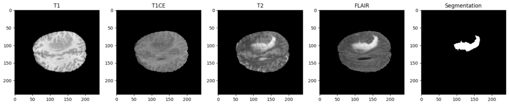
To be more specific, each patient of this dataset is represented through four different MRI scans / modalities, named T1, T1CE, T2 and FLAIR. These 4 images come with the ground truth segmentation of the tumoral and non-tumoral regions of their brains, which has been manually realized by experts.

Why 4 modalities ?

As you can see, the four modalities bring out different aspects for the same patient. To be more specific, here is a description of their interest:

• T1 : Show the structure and composition of different types of tissue.
• T1CE: Similar to T1 images but with the injection of a contrast agent, which will enhance the visibility of abnormalities.
• T2: Show the fluid content of different types of tissue.
• FLAIR: Used to suppress this fluid content, to better identify lesions and tumors that are not clearly visible on T1 or T2 images.

For an expert, it can be useful to have these 4 modalities in order to analyze the tumor more precisely, and to confirm its presence or not.

But for our artificial approach, using only two modalities instead of four is interesting since it can reduce the amount of manipulated data and therefore the computational and memory requirements of the segmentation task, making it faster and more efficient.

That is why we will exclude T1, since we have its improved version T1CE. Also, we will exclude the T2 modality. Indeed, the fluids it presents could degrade our predictions. These fluids are removed in the flair version, which highlights the affected regions much better, and will therefore be much more interesting for our training.

Images format

It is important to understand that all these MRI scans are NIfTI files (.nii format). A NIfTI image is a digital representation of a 3D object, such as a brain in our case. Indeed, our modalities and our annotations have a 3-dimensional (240, 240, 155) shape.

Each dimension is composed of a series of two-dimensional images, known as slices, which all contain the same number of pixels, and are stacked together to create a 3D representation. That is why we have been able to display 2D images just above. Indeed, we have displayed the 100th slice of a dimension for the 4 modalities and the segmentation.

Here is a quick presentation of these 3 planes:

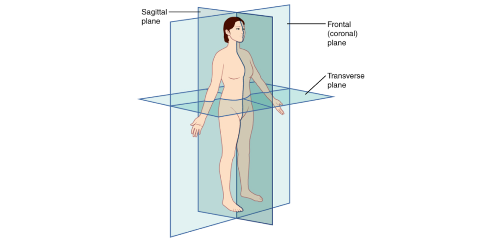
Planes of the body from Wikipedia Creative Commons

– Sagittal Plane: Divides the body into left and right sections and is often referred to as a “front-back” plane.

– Coronal Plane: Divides the body into front and back sections and is often referred to as a “side-side” plane.

– Axial or Transverse Plane: Divides the body into top and bottom sections and is often referred to as a “head-toe” plane.

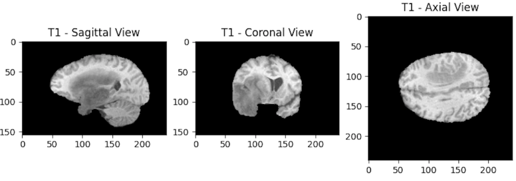
Each modality can then be displayed through its different planes. For example, we will display the 3 axes of the T1 modality:

Why choose to display the 100th slice?

Now that we know why we have three dimensions, let’s try to understand why we chose to display a specific slice.

To do this, we will display all the slices of a modality:

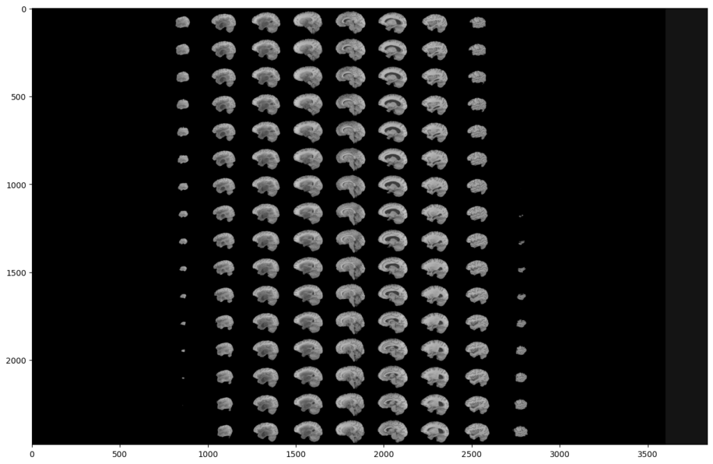
As you can see, two black parts are present on each side of our montage. However, these black parts correspond to slices. This means that a large part of the slices does not contain much information. This is not surprising since the MRI scanner goes through the brain gradually.

This analysis is the same on all other modalities, all planes and also on the images segmented by the experts. Indeed, they were not able to segment the slices that do not contain much information.

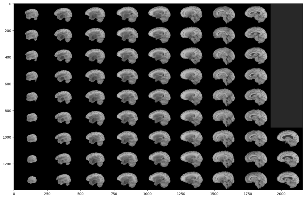
This is why we can exclude these slices in our analysis, in order to reduce the number of manipulated images, and speed up our training. Indeed, you can see that a (60:135) slices range will be much more interesting:

What about segmentations?

Now, let’s focus on the segmentations provided by the experts. What information do they give us?

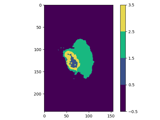
Regardless of the plane you are viewing, you will notice that some slices have multiple colors, which means that the experts have assigned multiple values / classes to the segmentation (one color represents one value).

Actually, we only have 4 possible pixels values in this dataset. These 4 values will form our 4 classes. Here is what they correspond to:

Class value	Class color	Class meaning
0	Purple	Not tumor (healthy zone or image background)
1	Blue	Necrotic and non-enhancing tumor
2	Green	Peritumoral Edema
4	Yellow	Enhancing Tumor

Explanation of the BraTS2020 dataset classes

As you can see, class 3 does not exist. We go directly to 4. We will therefore modify this “error” before sending the data to our model.

Our goal is to predict and segment each of these 4 classes for new patients to find out whether or not they have a brain tumor and which areas are affected.

To summarize data exploration:

• We have for each patient 4 different modalities (T1, T1CE, T2 & FLAIR), accompanied by a segmentation that indicates tumor areas.
• Modalities T1CE and FLAIR are the more interesting to keep, since these 2 provide complementary information about the anatomy and tissue contrast of the patient’s brain.
• Each image is 3D, and can therefore be analyzed through 3 different planes that are composed of 2D slices.
• Many slices contain little or no information. We will only keep the (60:135) slices range.
• A segmentation image contains 1 to 4 classes.
• Class number 4 must be reassigned to 3 since value 3 is missing.

Now that we know more about our data, it is time to prepare the training of our model.

2 – Training preparation

Split data into 3 sets

In the world of AI, the quality of a model is determined by its ability to make accurate predictions on new, unseen data. To achieve this, it is important to divide our data into three sets: Training, Validation and Test.

Reminder of their usefulness:

• Training set is used to train the model. During training, the model is exposed to the training data and adjusts its parameters to minimize the error between its predictions and the Ground truth (original segmentations).
• Validation set is used to fine-tune the hyperparameters of our model, which are set before training and determine the behavior of our model. The aim is to compare different hyperparameters and select the best configuration for our model.
• Test set is used to evaluate the performance of our model after it has been trained, to see how well it performs on data that was not used during the training of the model.

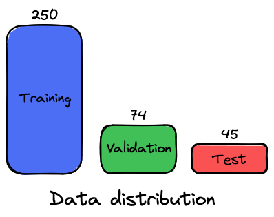
The dataset contains 369 different patients. Here is the distribution chosen for the 3 data sets:

Data preprocessing

In order to train a neural network to segment objects in images, it is necessary to feed it with both the raw image data (X) and the ground truth segmentations (y). By combining these two types of data, the neural network can learn to recognize tumor patterns and make accurate predictions about the contents of a patient’s scan.

Unfortunately, our modalities images (X) and our segmentations (y) cannot be sent directly to the AI model. Indeed, loading all these 3D images would overload the memory of our environment, and will lead to shape mismatch errors. We have to do some image preprocessing before, which will be done by using a Data Generator, where we will perform any operation that we think is necessary when loading the images.

As we have explained, we will, for each sample:

• Retrieve the paths of its 2 selected modalities (T1CE & FLAIR) and of its ground truth (original segmentation)
• Load modalities & segmentation
• Create a X array (image) that will contain all the selected slices (60-135) of these 2 modalities.
• Generate an y array (image) that will contain all the selected slices (60-135) of the ground truth.
• Assign to all the 4 in the y array the value 3 (in order to correct the class 3 missing case).

In addition to these preprocessing steps, we will:

Work in the axial plane

Since the images are square in shape (240×240) in this plane. But since we will manipulate a range of slices, we will be able to visualize the predictions in the 3 planes, so it doesn’t really have an impact.

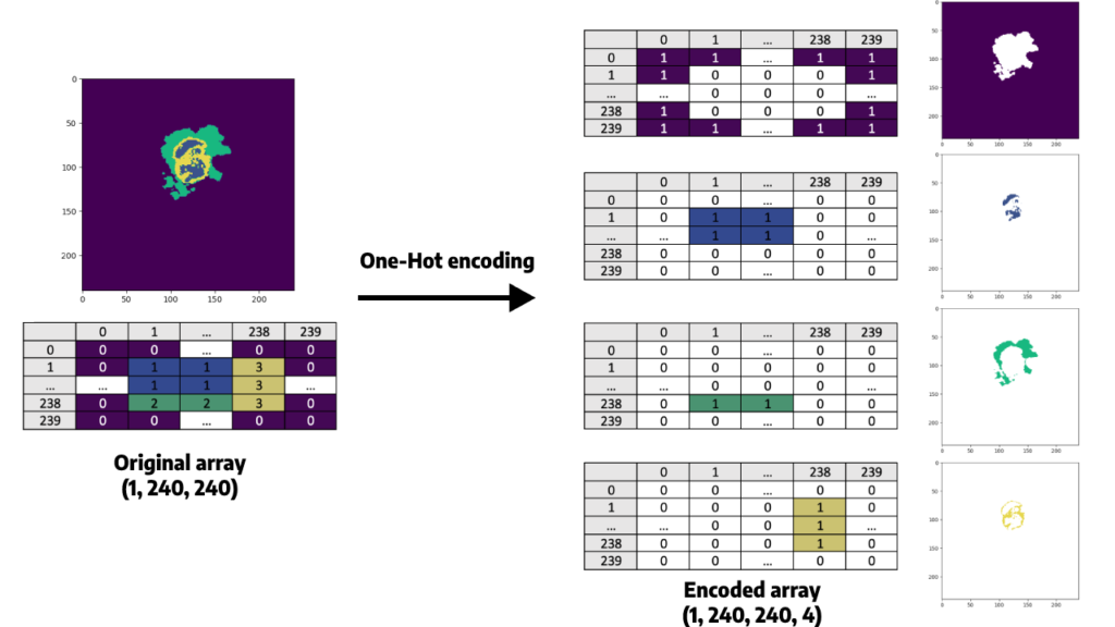
Apply a One-Hot Encoder to the y array

Since our goal is to segment regions that are represented as different classes (0 to 3), we must use One-Hot Encoding to convert our categorical variables (classes) into a numerical representation that can be used by our neural network (since they are based on mathematical equations).

Indeed, from a mathematical point of view, sending the y array as it is would mean that some classes are superior to others, while there is no superiority link between them. For example, class 1 is inferior to class 4 since 1 < 4. A One-Hot encoder will allow us to manipulate only 0 and 1.

Here is what it consists of, for one slice:

Resize each slice of our images from (240×240) to a (128, 128) shape.

Resizing is needed since we need image shapes that are a power of two (2ⁿ, where n is an integer). This is due to the fact that we will use pooling layers (MaxPooling2D) in our convolutional neural network (CNN), which reduce the spatial resolution by 2.

You may wonder why we didn’t resize the images in a (256, 256) shape, which also is a power of 2 and is closer to 240 than 128 is.

Indeed, resizing images to (256, 256) may preserve more information than resizing to (128, 128), which could lead to better performance. However, this larger size also means that the model will have more parameters, which will increase the training time and memory requirements. This is why we will choose the (128, 128) shape.

To summarize the preprocessing steps:

• We use a data generator to be able to process and send our data to our neural network (since all our images cannot be stored in memory at once).
• For each epoch (single pass of the entire training dataset through a neural network), the model will receive 250 samples (those contained in our training dataset).
• For each sample, the model will have to analyze 150 slices (since there are two modalities, and 75 selected slices for both of them), received in a (128, 128) shape, as an X array of a (128, 128, 75, 2) shape. This array will be provided with the ground truth segmentation of the patient, which will be One-Hot encoded and will then have a (75, 128, 128, 4) shape.

3 – Define the model

Now that our data is ready, we can define our segmentation model.

U-Net

We will use the U-Net architecture. This convolutional neural network (CNN) is designed for biomedical image segmentation, and is particularly well-suited for segmentation tasks where the regions of interest are small and have complex shapes (such as tumors in MRI scans).

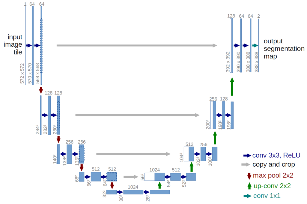
This neural network was first introduced in 2015 by Olaf Ronneberger, Philipp Fischer, Thomas Brox and reported in the paper U-Net: Convolutional Networks for Biomedical Image Segmentation.

Loss function

When training a CNN, it’s important to choose a loss function that accurately reflects the performance of the network. Indeed, this function will allow to compare the predicted pixels to those of the ground truth for each patient. At each epoch, the goal is to update the weights of our model in a way that minimizes this loss function, and therefore improves the accuracy of its predictions.

A commonly used loss function for multi-class classification problems is categorical cross-entropy, which measures the difference between the predicted probability distribution of each pixel and the real value of the one-hot encoded ground truth. Note that segmentations models sometimes use the dice loss function as well.

Output activation function

To get this probability distribution over the different classes for each pixel, we apply a softmax activation function to the output layer of our neural network.

This means that during training, our CNN will adjust its weights to minimize our loss function, which compares predicted probabilities given by the softmax function with those of the ground truth segmentation.

Other metrics

It is also important to monitor the model’s performance using evaluation metrics.

We will of course use accuracy, which is a very popular measure. However, this metric can be misleading when working with imbalanced datasets like BraTS2020, where Background class is over represented. To address this issue, we will use other metrics such as the intersection over union (IoU), the Dice coefficient, precision, sensitivity, and specificity.

• Accuracy: Measures the overall proportion of correctly classified pixels, including both positive and negative pixels.
• IoU: Measures the overlap between the predicted and ground truth segmentations.
• Precision (positive predictive value): Measures the proportion of predicted positive pixels that are actually positive.
• Sensitivity (true positive rate): Measures the proportion of positive ground truth pixels that were correctly predicted as positive.
• Specificity (true negative rate): Measures the proportion of negative ground truth pixels that were correctly predicted as negative.

4 – Analysis of training metrics

Model has been trained on 35 epochs.

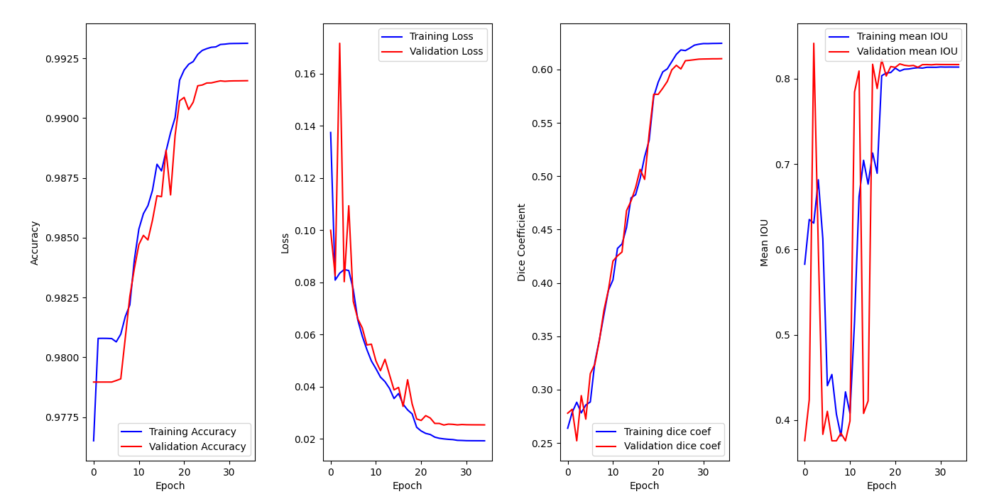
On the accuracy graph, we can see that both training accuracy and validation accuracy are increasing over epochs and reaching a plateau. This indicates that the model is learning from the data (training set) and generalizing well to new one (validation set). It does not seem that we are facing overfitting since both metrics are improving.

Then, we can see that our models is clearly learning from the training data, since both losses decrease over time on the second graph. We also notice that the best version of our model is reached around epoch 26. This conclusion is reinforced by the third graph, where both dice coefficients are increasing over epochs.

5 – Segmentation results

Once the training is completed, we can look at how the model behaves against the test set by calling the .evaluate() function:

Metric	Score
Categorical cross-entropy loss	0.0206
Accuracy	0.9935
MeanIOU	0.8176
Dice coefficient	0.6008
Precision	0.9938
Sensitivity	0.9922
Specificity	0.9979

We can conclude that the model performed very well on the test dataset, achieving a low test loss (0.0206), a correct dice coefficient (0.6008) for an image segmentation task, and good scores on other metrics which indicate that the model has good generalization performance on unseen data.

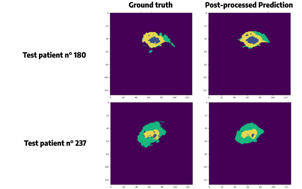
To understand a little better what is behind these scores, let’s try to plot some randomly selected patient predicted segmentations:

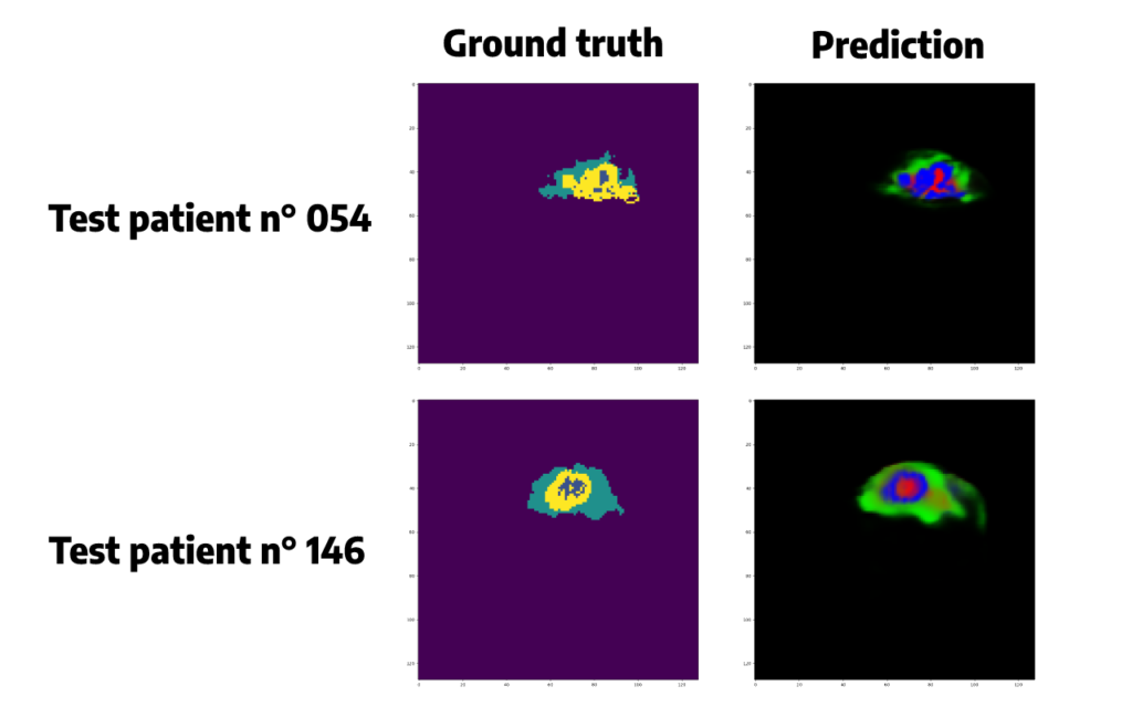
Predicted segmentations seem quite accurate but we need to do some post-processing in order to convert the probabilities given by the softmax function in a single class, for each pixel, corresponding to the class that has obtained the highest probability.

Argmax() function is chosen here. Applying this function will also allow us to remove some false positive cases, and to plot the same colors between the original segmentation and the prediction, which will be easier to compare than just above.

For the same patients as before, we obtain:

Conclusion

I hope you have enjoyed this tutorial, you are now more comfortable with image segmentation!

Keep in mind that even if our results seem accurate, we have some false positive in our predictions. In a field like medical imaging, it is crucial to evaluate the balance between true positives and false positives and assess the risks and benefits of an artificial approach.

As we have seen, post-processing techniques can be used to solve this problem. However, we must be careful with the results of these methods, since they can lead to a loss of information.

Want to find out more?

• Notebook

All the code is available on our GitHub repository.

• App

A Streamlit application was created around this use case to predict and observe the predictions generated by the model. Find the segmentation app’s code here.