Deploy a custom Docker image for Data Science project – Streamlit app for EDA and interactive prediction (Part 2)

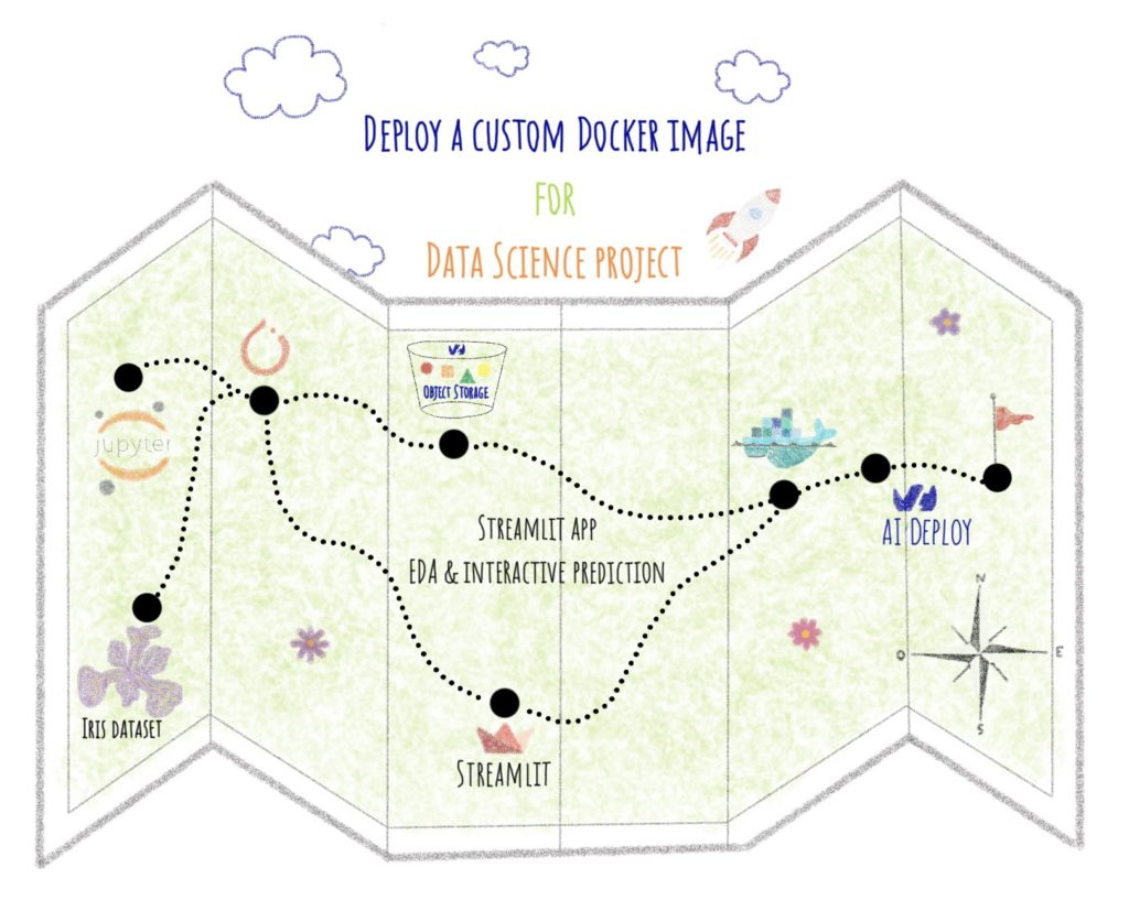
A guide to deploy a custom Docker image for a Streamlit app with AI Deploy.

Welcome to the second article concerning custom Docker image deployment. If you haven’t read the previous one, you can read it on the following link. It was about Gradio and sketch recognition.

When creating code for a Data Science project, you probably want it to be as portable as possible. In other words, it can be run as many times as you like, even on different machines.

Unfortunately, it is often the case that a Data Science code works fine locally on a machine but gives errors during runtime. It can be due to different versions of libraries installed on the host machine.

To deal with this problem, you can use Docker.

The article is organized as follows:

• Objectives
• Concepts
• Load the trained PyTorch model
• Build the Streamlit app with Python
• Containerize your app with Docker
• Launch the app with AI Deploy

All the code for this blogpost is available in our dedicated GitHub repository. You can test it with OVHcloud AI Deploy tool, please refer to the documentation to boot it up.

Objectives

In this article, you will learn how to develop Streamlit app for two Data Science tasks: Exploratory Data Analysis (EDA) and prediction based on ML model.

Once your app is up and running locally, it will be a matter of containerizing it, then deploying the custom Docker image with AI Deploy.

Concepts

In Artificial Intelligence, you probably hear about the famous use case of the Iris dataset. How about learning more about the iris dataset?

Iris dataset

Iris Flower Dataset is considered as the Hello World for Data Science. The Iris Flower Dataset contains four features (length and width of sepals and petals) of 50 samples of three species of Iris:

• Iris setosa
• Iris virginica
• Iris versicolor

The dataset is in csv format and you can also find it directly as a dataframe. It contains five columns namely:

• Petal length
• Petal width
• Sepal length
• Sepal width
• Species type

The objective of the models based on this dataset is to classify the three Iris species. The measurements of petals and sepals are used to create, for example, a linear discriminant model to classify species.

❗ A model to classify Iris species was trained in a previous tutorial, in notebook form, which you can find and test here.

This model is registered in an OVHcloud Object Storage container.

In this article, the first objective is to create an app for Exploratory Data Analysis (EDA). Then you will see how to obtain interactive prediction.

EDA

What is EDA in Data Science?

Exploratory Data Analysis (EDA) is a technique to analyze data with visual techniques. In this way, you have detailed information about the statistical summary of the data.

In addition, EDA allows duplicate values, outliers to be dealt with, and also to see certain trends or patterns present in the dataset.

For Iris dataset, the aim is to observe the source data on visual graphs using the Streamlit tool.

Streamlit

What is Streamlit?

Streamlit allows you to transform data scripts into quickly shareable web applications using only the Python language. Moreover, this framework does not require front-end skills.

This is a time saver for the data scientist who wants to deploy an app around the world of data!

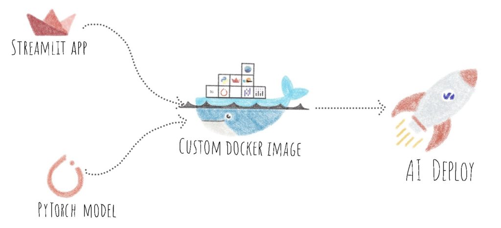
To make this app accessible, you need to containerize it using Docker.

Docker

Docker platform allows you to build, run and manage isolated applications. The principle is to build an application that contains not only the written code but also all the context to run the code: libraries and their versions for example

When you wrap your application with all its context, you build a Docker image, which can be saved in your local repository or in the Docker Hub.

To get started with Docker, please, check this documentation.

To build a Docker image, you will define 2 elements:

• the application code (Streamlit app)
• the Dockerfile

In the next steps, you will see how to develop the Python code for your app, but also how to write the Dockerfile.

Finally, you will see how to deploy your custom docker image with OVHcloud AI Deploy tool.

AI Deploy

AI Deploy enables AI models and managed applications to be started via Docker containers.

To know more about AI Deploy, please refer to this documentation.

Load the trained PyTorch model

❗ To develop an app that uses a machine learning model, you must first load the model in the correct format. For this tutorial, a PyTorch model is used and the Python file utils.py is used to load it.

The first step is to import the Python libraries needed to load a PyTorch model in the utils.py file.

import torch
import torch.nn as nn
import torch.nn.functional as F

To load your PyTorch model, it is first necessary to define its model architecture by using the Model class defined previously in the part “Step 2 – Define the neural network model” of the notebook.

class Model(nn.Module):
    def __init__(self):

        super().__init__()
        self.layer1 = nn.Linear(in_features=4, out_features=16)
        self.layer2 = nn.Linear(in_features=16, out_features=12)
        self.output = nn.Linear(in_features=12, out_features=3)

    def forward(self, x):

        x = F.relu(self.layer1(x))
        x = F.relu(self.layer2(x))
        x = self.output(x)

        return x

In a second step, you fill in the access path to the model. To save this model in pth format, refer to the part “Step 6 – Save the model for future inference” of the notebook.

path = "model_iris_classification.pth"

Then, the load_checkpoint function is used to load the model’s checkpoint.

def load_checkpoint(path):

    model = Model()
    print("Model display: ", model)
    model.load_state_dict(torch.load(path))
    model.eval()

    return model

Finally, the function load_model is used to load the model and to use it to obtain the result of the prediction.

def load_model(X_tensor):

    model = load_checkpoint(path)
    predict_out = model(X_tensor)
    _, predict_y = torch.max(predict_out, 1)

    return predict_out.squeeze().detach().numpy(), predict_y.item()

Find out the full Python code here.

Have you successfully loaded your model? Good job 🥳 !

Let’s go for the creation of the Streamlit app!

Build the Streamlit app with Python

❗ All the codes below are available in the app.py file. The key functions are explained in this article.
However, the "main" part of the app.py file is not described. You can find the complete Python code of the app.py file here.

To begin, you can import dependencies for Streamlit app.

• Numpy
• Pandas
• Seaborn
• load_model function from utils.py
• Torch
• Streamlit
• Scikit-Learn
• Ploty
• PIL

import numpy as np
import pandas as pd
import seaborn as sns
from utils import load_model
import torch
import streamlit as st
from sklearn.datasets import load_iris
from sklearn.decomposition import PCA
import plotly.graph_objects as go
import plotly.express as px
from PIL import Image

Then, you must load source dataset of Iris flowers to be able to extract the characteristics and thus, visualize data. Scikit-Learn allows to load this dataset without having to download it!

Next, you can separate the dataset in an input dataframe and an output dataframe.

Finally, this load_data function is cached so that you don’t have to download again the dataset.

@st.cache
def load_data():
    dataset_iris = load_iris()
    df_inputs = pd.DataFrame(dataset_iris.data, columns=dataset_iris.feature_names)
    df_output = pd.DataFrame(dataset_iris.target, columns=['variety'])

    return df_inputs, df_output

The creation of this Streamlit app is separated into two parts.

Firstly, you can look into the creation of the EDA part. Then you will see how to create an interactive prediction tool using the PyTorch model.

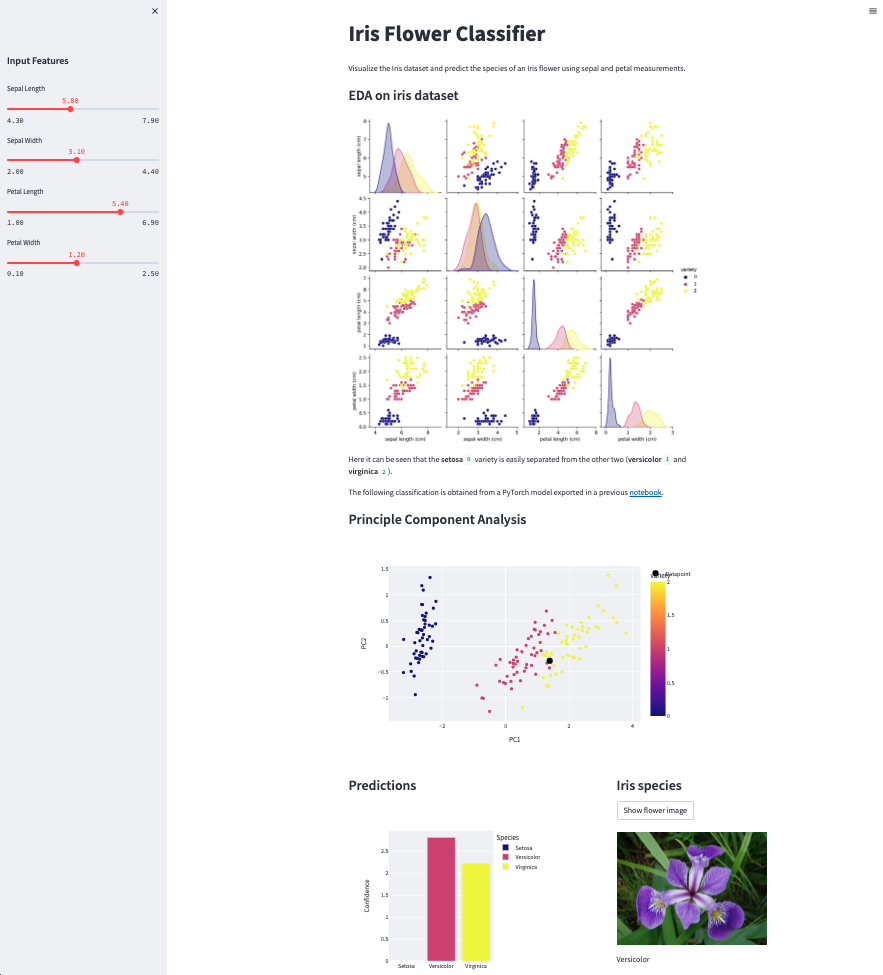
EDA on Iris Dataset

As a first step, you can look at the source dataset by displaying different graphs using the Python Seaborn library.

Seaborn Pairplot allows you to get the relationship between each variable present in Pandas dataframe.

sns.pairplot plots the graph in pairs of several features in a grid format.

@st.cache(allow_output_mutation=True)
def data_visualization(df_inputs, df_output):

    df = pd.concat([df_inputs, df_output['variety']], axis=1)
    eda = sns.pairplot(data=df, hue="variety", palette=['#0D0888', '#CB4779', '#F0F922'])

    return eda

Later, this function will display the following graph thanks to a call in the “main” of app.py file.

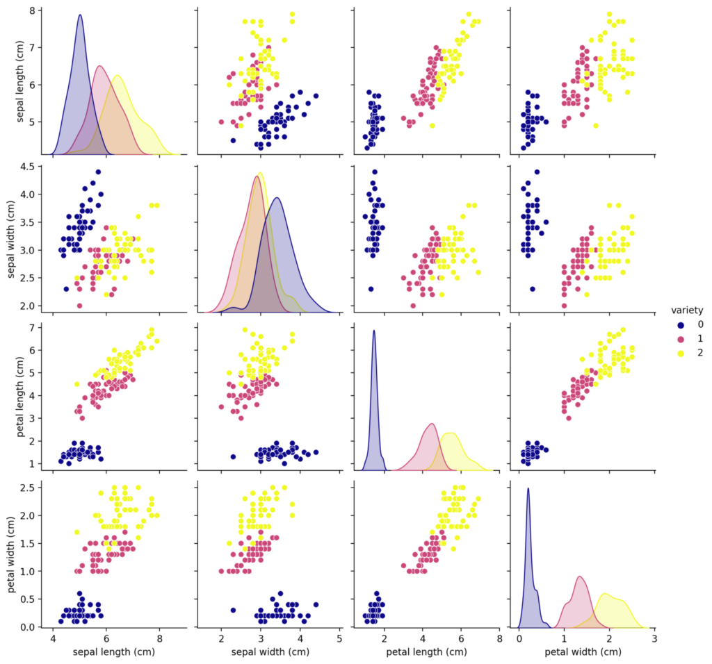
Here it can be seen that the setosa 0 variety is easily separated from the other two (versicolor 1 and virginica 2).

Were you able to display your graph? Well done 🎉 !

So, let’s go to the interactive prediction tool 🔜 !

Create an interactive prediction tool

To create an interactive prediction tool, you will need several elements:

• Firstly, you need four sliders to play with the input parameters
• Secondly, you have to create a function to display the Principal Component Analysis (PCA) graph to visualize the point corresponding to the output of the model
• Thirdly, you can build a histogram representing the result of the prediction
• Fourthly, you will have a function to display the image of the predicted Iris species

Ready to go? Let’s start creating sliders!

Create a sidebar with sliders for input data

In order to facilitate the visual reading of the Streamlit app, sliders are added in a sidebar.

In this sidebar, four sliders are added so that users can choose the length and width of petals and sepals.

How to create a slider? Well, nothing could be easier than with Streamlit!

You need to define the function st.sidebar.slider() to add a slider to the sidebar. Then you can specify arguments such as minimum and maximum values or the average value which will be the default value. Finally, you can specify the step of your slider.

❗ Here you can see the example for a single slider. Find the complete code of the other sliders on the GitHub repo here.

def create_slider(df_inputs):

    sepal_length = st.sidebar.slider(
        label='Sepal Length',
        min_value=float(df_inputs['sepal length (cm)'].min()),
        max_value=float(df_inputs['sepal length (cm)'].max()),
        value=float(round(df_inputs['sepal length (cm)'].mean(), 1)),
        step=0.1)

    sepal_width = st.sidebar.slider(
        ...
        )

    petal_length = st.sidebar.slider(
        ...
        )

    petal_width = st.sidebar.slider(
        ...
        )

    return sepal_length, sepal_width, petal_length, petal_width

Later, this function will be call in the “main” of the app.py file. Afterwards, you will see the following interface:

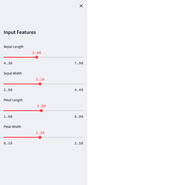
Thanks to these sliders, you can now obtain the result of the prediction in an interactive way by playing on one or more parameters.

Display PCA graph

Once your sliders are up and running, you can create a function to display the graph of the Principal Component Analysis (PCA).

PCA is a technique that transforms high-dimensional data into lower dimensions while retaining as much information as possible.

What about the Iris dataset? The aim is to be able to display the point resulting from the model prediction on a two-dimensional graph.

The run_pca function below displays the two-dimensional graph with iris of the source dataset.

@st.cache
def run_pca():

    pca = PCA(2)
    X = df_inputs.iloc[:, :4]
    X_pca = pca.fit_transform(X)
    df_pca = pd.DataFrame(pca.transform(X))
    df_pca.columns = ['PC1', 'PC2']
    df_pca = pd.concat([df_pca, df_output['variety']], axis=1)

    return pca, df_pca

Thereafter, the black point corresponding to the result of the prediction is placed on the same graph in the “main” of the Python app.py file.

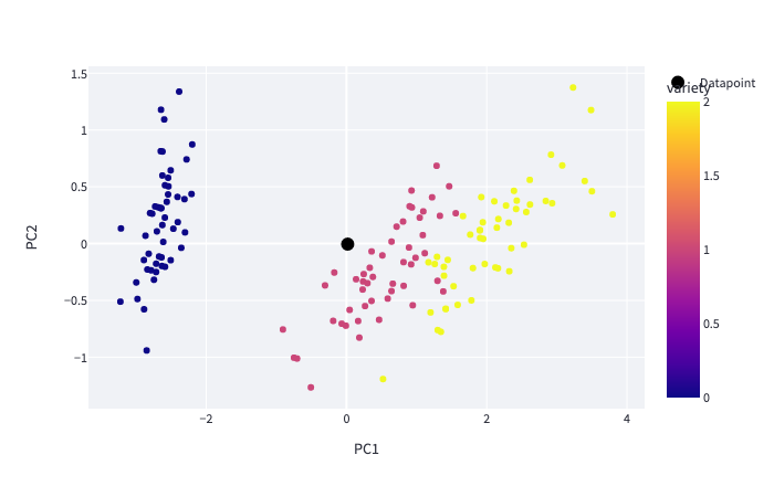
With this method you were able to visualize your point in space. However, the numerical result of the prediction is not filled in.

Therefore, you can also display the results as a histogram.

Return predictions histogram

At the output of the neural network, the results can be positive or negative and the highest value corresponds to the iris species predicted by the model.

To create a histogram, negative values can be removed. To do this, the predictions with positive values are extracted and sent to a list before being transformed into a dataframe.

The negative values are all replaced by the null value.

To summarize, the extract_positive_value function can be translated into the following mathematical formula:
f(prediction) = max(0, prediction)

def extract_positive_value(prediction):

    prediction_positive = []
    for p in prediction:
        if p < 0:
            p = 0
        prediction_positive.append(p)

    return pd.DataFrame({'Species': ['Setosa', 'Versicolor', 'Virginica'], 'Confidence': prediction_positive})

This function is then called to build the histogram in the “main” of the Python app.py file. The library plotly allows to build this bar chart as follows.

fig = px.bar(extract_positive_value(prediction), x='Species', y='Confidence', width=400, height=400, color='Species', color_discrete_sequence=['#0D0888', '#CB4779', '#F0F922'])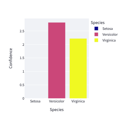

Show Iris species image

The final step is to display the predicted iris image using a Streamlit button. Therefore, you can define the display_image function to select the correct image based on the prediction.

def display_img(species):

    list_img = ['setosa.png', 'versicolor.png', 'virginica.png']

    return Image.open(list_img[species])

Finally, in the main Python code app.py, st.image() displays the image when the user requests it by pressing the “Show flower image” button.

if st.button('Show flower image'):
    st.image(display_img(species), width=300)
    st.write(df_pred.iloc[species, 0])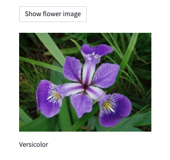

❗ Again, you can find the full code here.

Before deploying your Streamlit app, you can test it locally using the following command:

streamlit run app.py

Then, you can test your app locally at the following address: http://localhost:8080/

Your app works locally? Congratulations 🎉 !

Now it’s time to move on to containerization!

Containerize your app with Docker

First of all, you have to build the file that will contain the different Python modules to be installed with their corresponding version.

Create the requirements.txt file

The requirements.txt file will allow us to write all the modules needed to make our application work.

pandas==1.4.4
numpy==1.23.2
torch==1.12.1
streamlit==1.12.2
scikit-learn==1.1.2
plotly==5.10.0
Pillow==9.2.0
seaborn==0.12.0

This file will be useful when writing the Dockerfile.

Write the Dockerfile

Your Dockerfile should start with the the FROM instruction indicating the parent image to use. In our case we choose to start from a classic Python image.

For this Streamlit app, you can use version 3.8 of Python.

FROM python:3.8

Next, you have to to fill in the working directory and add all files into.

❗ Here you must be in the /workspace directory. This is the basic directory for launching an OVHcloud AI Deploy.

WORKDIR /workspace
ADD . /workspace

Install the requirements.txt file which contains your needed Python modules using a pip install… command:

RUN pip install -r requirements.txt

Then, you can give correct access rights to OVHcloud user (42420:42420).

RUN chown -R 42420:42420 /workspace
ENV HOME=/workspace

Finally, you have to define your default launching command to start the application.

CMD [ "streamlit", "run", "/workspace/app.py", "--server.address=0.0.0.0" ]

Once your Dockerfile is defined, you will be able to build your custom docker image.

Build the Docker image from the Dockerfile

First, you can launch the following command from the Dockerfile directory to build your application image.

docker build . -t streamlit-eda-iris:latest

⚠️ The dot . argument indicates that your build context (place of the Dockerfile and other needed files) is the current directory.

⚠️ The -t argument allows you to choose the identifier to give to your image. Usually image identifiers are composed of a name and a version tag <name>:<version>. For this example we chose streamlit-eda-iris:latest.

Test it locally

Now, you can run the following Docker command to launch your application locally on your computer.

docker run --rm -it -p 8501:8501 --user=42420:42420 streamlit-eda-iris:latest

⚠️ The -p 8501:8501 argument indicates that you want to execute a port redirection from the port 8501 of your local machine into the port 8501 of the Docker container.

⚠️ Don't forget the --user=42420:42420 argument if you want to simulate the exact same behaviour that will occur on AI Deploy. It executes the Docker container as the specific OVHcloud user (user 42420:42420).

Once started, your application should be available on http://localhost:8080.

Your Docker image seems to work? Good job 👍 !

It’s time to push it and deploy it!

Push the image into the shared registry

❗ The shared registry of AI Deploy should only be used for testing purpose. Please consider attaching your own Docker registry. More information about this can be found here.

Then, you have to find the address of your shared registry by launching this command.

ovhai registry list

Next, log in on the shared registry with your usual OpenStack credentials.

docker login -u <user> -p <password> <shared-registry-address>

To finish, you need to push the created image into the shared registry.

docker tag streamlit-eda-iris:latest <shared-registry-address>/streamlit-eda-iris:latest
docker push <shared-registry-address>/streamlit-eda-iris:latest

Once you have pushed your custom docker image into the shared registry, you are ready to launch your app 🚀 !

Launch the AI Deploy app

The following command starts a new job running your Streamlit application.

ovhai app run \
      --default-http-port 8501 \
      --cpu 12 \
      <shared-registry-address>/streamlit-eda-iris:latest

Choose the compute resources

First, you can either choose the number of GPUs or CPUs for your app.

--cpu 12 indicates that we request 12 CPUs for that app.

If you want, you can also launch this app with one or more GPUs.

Make the app public

Finally, if you want your app to be accessible without the need to authenticate, specify it as follows.

Consider adding the --unsecure-http attribute if you want your application to be reachable without any authentication.

Conclusion

Well done 🎉 ! You have learned how to build your own Docker image for a dedicated EDA and interactive prediction app!

You have also been able to deploy this app thanks to OVHcloud’s AI Deploy tool.

In a third article, you will see how it is possible to deploy a Data Science project with an API for Spam classification.

Want to find out more?

Notebook

You want to access the notebook? Refer to the GitHub repository.

App

You want to access to the full code to create the Streamlit app? Refer to the GitHub repository.

To launch and test this app with AI Deploy, please refer to our documentation.

References

• How to Run a Data Science Project in a Docker Container
• Create a Machine Learning Web App with Streamlit