
A guide to analyze and classify marine mammal sounds.
Since you're reading a blog post from a technology company, I bet you've heard about AI, Machine and Deep Learning many times before.
Audio or sound classification is a technique with multiple applications in the field of AI and data science.
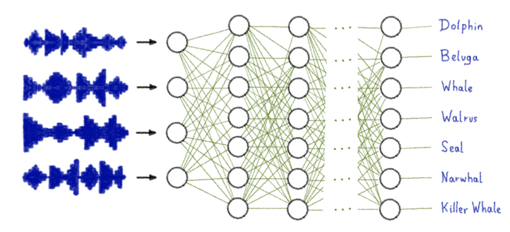
Use cases
- Acoustic data classification:
- identifies location
- differentiates environments
- has a role in ecosystem monitoring
- Environmental sound classification:
- recognition of urban sounds
- used in security system
- used in predictive maintenance
- used to differentiate animal sounds
- Music classification:
- classify music
- key role in: audio libraries organisation by genre, improvement of recommandation algorithms, discovery of trends, listener preferences through data analysis, ...
- Natural language classification:
- human speech classification
- common in: chatbots, virtual assistants, tech-to-speech application, ...
In this article we will look at the classification of marine mammal sounds.
Objective
The purpose of this article is to explain how to train a model to classify audios using AI Notebooks.
In this tutorial, the sounds in the dataset are in .wav format. To be able to use them and obtain results, it is necessary to pre-process this data by following different steps.
- Analyse one of these audio recordings
- Transform each sound file into a .csv file
- Train your model from the .csv file
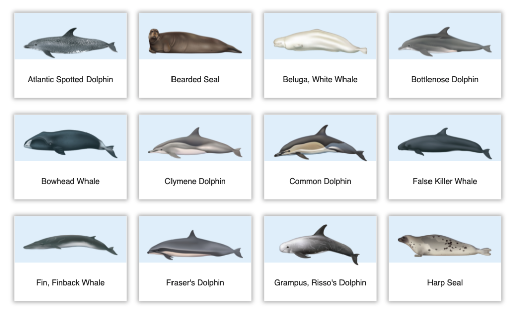
This dataset is composed of 55 different folders corresponding to the marine mammals. In each folder are stored several sound files of each animal.
You can get more information about this dataset on this website.
The data distribution is as follows:
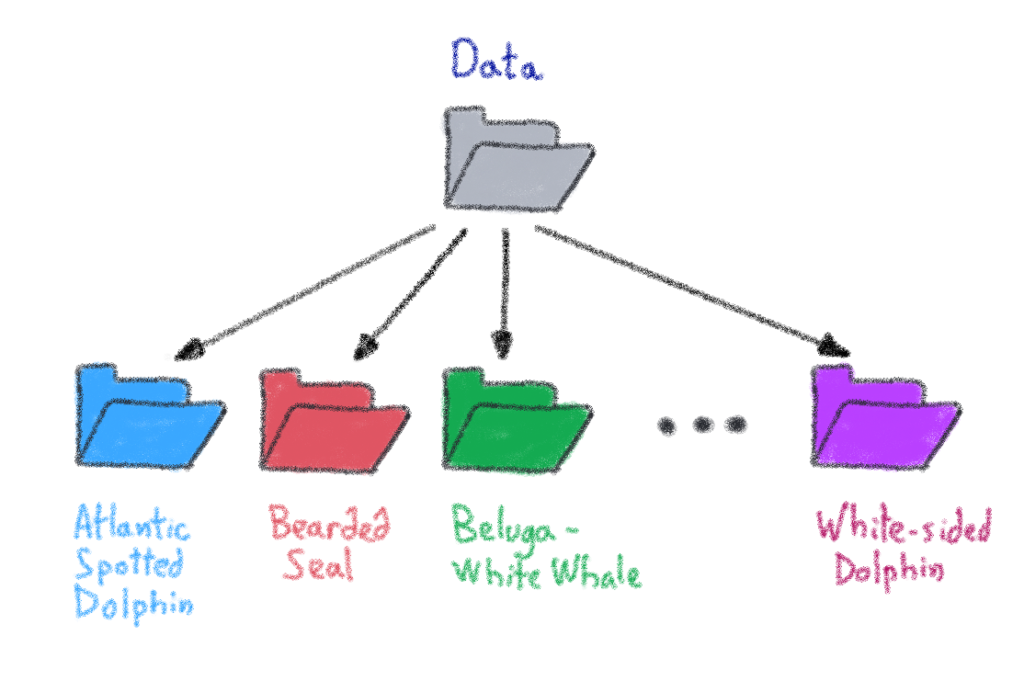
⚠️ For this example, we choose only the first 45 classes (or folders).
Let's follow the different steps!

Audio libraries
1. Loading an audio file with Librosa
Librosa is a Python module for audio signal analysis. By using Librosa, you can extract key features from the audio samples such as Tempo, Chroma Energy Normalized, Mel-Freqency Cepstral Coefficients, Spectral Centroid, Spectral Contrast, Spectral Rolloff, and Zero Crossing Rate. If you want to know more about this library, refer to the documentation.
import librosa
import librosa.display as lplt
You can start by looking at your data by displaying different parameters using the Librosa library.
First, you can do a test on a file.
test_sound = "data/AtlanticSpottedDolphin/61025001.wav"Loads and decodes the audio.
data, sr = librosa.load(test_sound)
print(type(data), type(sr))
<class 'numpy.ndarray'> <class 'int'>
librosa.load(test_sound ,sr = 45600)(array([-0.0739522 , -0.06588229, -0.06673266, ..., 0.03021295, 0.05592792, 0. ], dtype=float32), 45600)
2. Playing Audio with IPython.display.Audio
IPython.display.Audio advises you play audio directly in a Jupyter notebook.
Using IPython.display.Audio to play the audio.
import IPython

IPython.display.Audio(data, rate = sr)
Visualizing Audio
1. Waveforms
Waveforms are visual representations of sound as time on the x-axis and amplitude on the y-axis. They allow for quick analysis of audio data.
We can plot the audio array using librosa.display.waveplot.
plt.show(librosa.display.waveplot(data))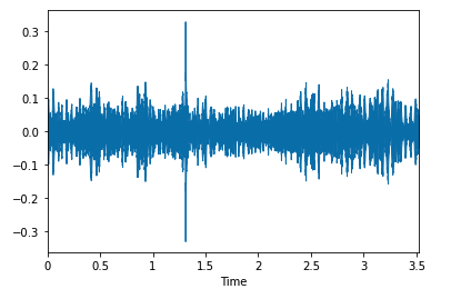
2. Spectrograms
A spectrogram is a visual way of representing the intensity of a signal over time at various frequencies present in a particular waveform.
stft = librosa.stft(data)
plt.colorbar(librosa.display.specshow(stft, sr = sr, x_axis = 'time', y_axis = 'hz'))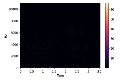
stft_db = librosa.amplitude_to_db(abs(stft))
plt.colorbar(librosa.display.specshow(stft_db, sr = sr, x_axis = 'time', y_axis = 'hz'))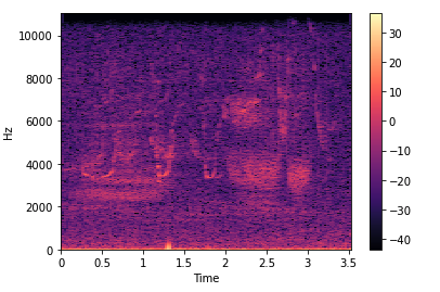
3. Spectral Rolloff
Spectral Rolloff is the frequency below which a specified percentage of the total spectral energy.
librosa.feature.spectral_rolloff calculates the attenuation frequency for each frame of a signal.
spectral_rolloff = librosa.feature.spectral_rolloff(data + 0.01, sr = sr)[0]
plt.show(librosa.display.waveplot(data, sr = sr, alpha = 0.4))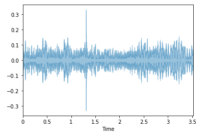
4. Chroma Feature
This tool is perfect for analyzing musical features whose pitches can be meaningfully categorized and whose tuning is close to the equal temperament scale.
chroma = librosa.feature.chroma_stft(data, sr = sr)
lplt.specshow(chroma, sr = sr, x_axis = "time" ,y_axis = "chroma", cmap = "coolwarm")
plt.colorbar()
plt.title("Chroma Features")
plt.show()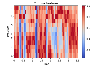
5. Zero Crossing Rate
A zero crossing occurs if successive samples have different algebraic signs.
- The rate at which zero crossings occur is a simple measure of the frequency content of a signal.
- The number of zero-crossings measures the number of times in a time interval that the amplitude of speech signals passes through a zero value.
start = 1000
end = 1200
plt.plot(data[start:end])
plt.grid()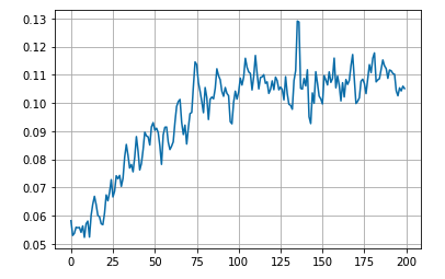
Data preprocessing
1. Data transformation
To train your model, preprocessing of data is required. First of all, you have to convert the .wav into a .csv file.
- Define columns name:
header = "filename length chroma_stft_mean chroma_stft_var rms_mean rms_var spectral_centroid_mean spectral_centroid_var spectral_bandwidth_mean spectral_bandwidth_var rolloff_mean rolloff_var zero_crossing_rate_mean zero_crossing_rate_var harmony_mean harmony_var perceptr_mean perceptr_var tempo mfcc1_mean mfcc1_var mfcc2_mean mfcc2_var mfcc3_mean mfcc3_var mfcc4_mean mfcc4_var label".split()- Create the data.csv file:
import csv

file = open('data.csv', 'w', newline = '')
with file:
    writer = csv.writer(file)
writer.writerow(header)- Define character string of marine mammals (45):
There are 45 different marine animals, or 45 classes.
marine_mammals = "AtlanticSpottedDolphin BeardedSeal Beluga_WhiteWhale BlueWhale BottlenoseDolphin Boutu_AmazonRiverDolphin BowheadWhale ClymeneDolphin Commerson'sDolphin CommonDolphin Dall'sPorpoise DuskyDolphin FalseKillerWhale Fin_FinbackWhale FinlessPorpoise Fraser'sDolphin Grampus_Risso'sDolphin GraySeal GrayWhale HarborPorpoise HarbourSeal HarpSeal Heaviside'sDolphin HoodedSeal HumpbackWhale IrawaddyDolphin JuanFernandezFurSeal KillerWhale LeopardSeal Long_FinnedPilotWhale LongBeaked(Pacific)CommonDolphin MelonHeadedWhale MinkeWhale Narwhal NewZealandFurSeal NorthernRightWhale PantropicalSpottedDolphin RibbonSeal RingedSeal RossSeal Rough_ToothedDolphin SeaOtter Short_Finned(Pacific)PilotWhale SouthernRightWhale SpermWhale".split()- Transform each .wav file into a .csv row:
for animal in marine_mammals:

  for filename in os.listdir(f"/workspace/data/{animal}/"):

    sound_name = f"/workspace/data/{animal}/{filename}"
    y, sr = librosa.load(sound_name, mono = True, duration = 30)
    chroma_stft = librosa.feature.chroma_stft(y = y, sr = sr)
    rmse = librosa.feature.rms(y = y)
    spec_cent = librosa.feature.spectral_centroid(y = y, sr = sr)
    spec_bw = librosa.feature.spectral_bandwidth(y = y, sr = sr)
    rolloff = librosa.feature.spectral_rolloff(y = y, sr = sr)
    zcr = librosa.feature.zero_crossing_rate(y)
    mfcc = librosa.feature.mfcc(y = y, sr = sr)
    to_append = f'{filename} {np.mean(chroma_stft)} {np.mean(rmse)} {np.mean(spec_cent)} {np.mean(spec_bw)} {np.mean(rolloff)} {np.mean(zcr)}'

    for e in mfcc:
        to_append += f' {np.mean(e)}'

    to_append += f' {animal}'
    file = open('data.csv', 'a', newline = '')

    with file:
        writer = csv.writer(file)
writer.writerow(to_append.split())- Display the data.csv file:
df = pd.read_csv('data.csv')2. Features extraction
In the preprocessing of the data, feature extraction is necessary before running the training. The purpose is to define the inputs and outputs of the neural network.
- OUTPUT (y): last column which is the label.
You cannot use text directly for training. You will encode these labels with the LabelEncoder() function of sklearn.preprocessing.
Before running a model, you need to convert this type of categorical text data into numerical data that the model can understand.
from sklearn.preprocessing import LabelEncoder

class_list = df.iloc[:,-1]
converter = LabelEncoder()
y = converter.fit_transform(class_list)
print("y: ", y)
y : [ 0 0 0 ... 44 44 44]
- INPUTS (X): all other columns are input parameters to the neural network.
Remove the first column which does not provide any information for the training (the filename) and the last one which corresponds to the output.
from sklearn.preprocessing import StandardScaler

fit = StandardScaler()
X = fit.fit_transform(np.array(df.iloc[:, 1:26], dtype=float))
3. Split dataset for training
from sklearn.model_selection import train_test_split

X_train, X_test, y_train, y_test = train_test_split(X, y, test_size = 0.2)
Building the model
The first step is to build the model and display the summary.
For the CNN model, all hidden layers use a ReLU activation function, the output layer a Softmax function and a Dropout is used to avoid overfitting.
import keras
import tensorflow as tf
from tensorflow.keras.models import Sequential

model = tf.keras.models.Sequential([
    tf.keras.layers.Dense(512, activation = 'relu', input_shape = (X_train.shape[1],)),
    tf.keras.layers.Dropout(0.2),

    tf.keras.layers.Dense(256, activation = 'relu'),
    keras.layers.Dropout(0.2),

    tf.keras.layers.Dense(128, activation = 'relu'),
    tf.keras.layers.Dropout(0.2),

    tf.keras.layers.Dense(64, activation = 'relu'),
    tf.keras.layers.Dropout(0.2),

    tf.keras.layers.Dense(45, activation = 'softmax'),
])

print(model.summary())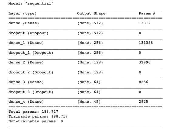
Model training and evaluation
Adam optimizer is used to train the model over 100 epochs. This choice was made because it allows us to obtain better results.
The loss is calculated with the sparse_categorical_crossentropy function.
def trainModel(model,epochs, optimizer):
    batch_size = 128
    model.compile(optimizer = optimizer, loss = 'sparse_categorical_crossentropy', metrics = 'accuracy')
    return model.fit(X_train, y_train, validation_data = (X_test, y_test), epochs = epochs, batch_size = batch_size)
Now, launch the training!
model_history = trainModel(model = model, epochs = 100, optimizer = 'adam')- Display loss curves
loss_train_curve = model_history.history["loss"]
loss_val_curve = model_history.history["val_loss"]
plt.plot(loss_train_curve, label = "Train")
plt.plot(loss_val_curve, label = "Validation")
plt.legend(loc = 'upper right')
plt.title("Loss")
plt.show()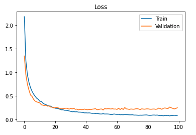
- Display accuracy curves
acc_train_curve = model_history.history["accuracy"]
acc_val_curve = model_history.history["val_accuracy"]
plt.plot(acc_train_curve, label = "Train")
plt.plot(acc_val_curve, label = "Validation")
plt.legend(loc = 'lower right')
plt.title("Accuracy")
plt.show()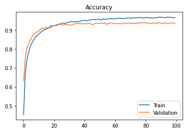
test_loss, test_acc = model.evaluate(X_test, y_test, batch_size = 128)
print("The test loss is: ", test_loss)
print("The best accuracy is: ", test_acc*100)
20/20 [==============================] - 0s 3ms/step - loss: 0.2854 - accuracy: 0.9371 The test loss is: 0.24700121581554413The best accuracy is: 93.71269345283508
Save the model for future inference
1. Save and store the model in an OVHcloud Object Container
model.save('/workspace/model-marine-mammal-sounds/saved_model/my_model')You can check your model directory.
%ls /workspace/model-marine-mammal-sounds/saved_modelSaved_model contains an assets folder, saved_model.pb, and variables folder.
%ls /workspace/model-marine-mammal-sounds/saved_model/my_modelThen, you are able to load this model.
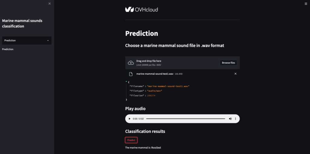
model = tf.keras.models.load_model('/workspace/model-marine-mammal-sounds/saved_model/my_model')Do you want to use this model in a Streamlit app? Refer to our GitHub repository.
Conclusion
The accuracy of the model can be improved by increasing the number of epochs, but after a certain period we reach a threshold, so the value should be determined accordingly.
The accuracy obtained for the test set is 93.71 %, which is a satisfactory result.
Want to find out more?
If you want to access the notebook, refer to the GitHub repository.
To launch and test this notebook with AI Notebooks, please refer to our documentation.
You can also look at this presentation done at a OVHcloud Startup Program event at Station F:
I hope you have enjoyed this article. Try for yourself!