A journey into the wondrous land of Machine Learning, or “Cleaning data is funnier than cleaning my flat!” (Part 3)

What am I doing here?

The story so far…

As you might know if you have read our blog for more than a year, a few years ago, I bought a flat in Paris. If you don’t know, the real estate market in Paris is expensive but despite that, it is so tight that a good flat at a correct price can be for sale for less than a day.

Obviously, you have to take a decision quite fast, and considering the prices, you have to trust your decision. Of course, to trust your decision, you have to take your time, study the market, make some visits etc… This process can be quite long (in my case it took a year between the time I decided that I wanted to buy a flat and the time I actually commited to buying my current flat), and even spending a lot of time will never allow you to have a perfect understanding of the market. What if there was a way to do that very quickly and with a better accuracy than with the standard process?

As you might also know if you are one of our regular readers, I tried to solve this problem with Machine Learning, using an end-to-end software called Dataiku. In a first blog post, we learned how to make a basic use of Dataiku, and discovered that just knowing how to click on a few buttons wasn’t quite enough: you had to bring some sense in your data and in the training algorithm, or you would find absurd results.

In a second entry, we studied a bit more the data, tweaked a few parameters and values in Dataiku’s algorithms and trained a new model. This yielded a much better result, and this new model was – if not accurate – at least relevant: the same flat had a higher predicted place when it was bigger or supposedly in a better neighbourhood. However, it was far from perfect and really lacked accuracy for several reasons, some of them out of our control.

However, all of this was done on one instance of Dataiku – a licensed software – on a single VM. There are multiple reasons that could push me to do things differently:

• Maybe you want to only use open-source frameworks to make sure you have full control over exactly what runs and how it works
• Maybe you don’t want to pay a license to make an extensive use of the software
• Maybe you have a vast amount of data to process and transform and even a big VM is not enough
• Maybe you want to only use “universal” tools and languages to make sure you will always find people with the appropriate skills so that your pipelines are maintaineable

But seriously, what am I doing?

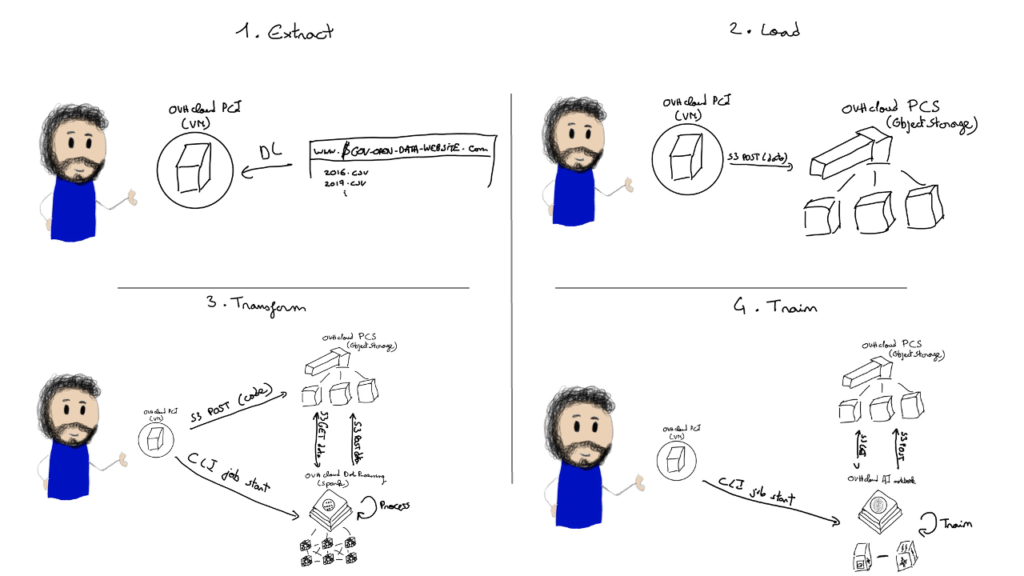
What we did very intuitively (and somewhat naively) with Dataiku was actually a quite complex pipeline that is often called ELT, for Extract, Load and Transform.

• We extracted the data when we downloaded it from the French open data website
• We loaded it when we uploaded it to our Dataiku Instance
• We transformed it when we used Dataiku’s data processing capabilities to make it digestible for a machine learning algorithm

And obviously, after this ELT process, we added a step to train a model on the transformed data.

So what are we going to do to redo all of that without Dataiku’s help?

• For the extract phase, we are actually going to cheat a little bit and do things the exact same way: we will download the data directly from the website on a public cloud VM. Obviously this is not very scalable, but the extract phase is the most dependant on the source format: in that case, it’s csv files from a webserver.
• For the load phase, we are going to push these csv files to an object store – in that case OVHcloud PCS (Public Cloud Storage) – using the standard S3 CLI. An object store is ideal to store this kind of data because:
  • It is infinitely scalable so no matter how much data I push, I won’t have to handle storage provisioning etc…
  • It works best with large objects (> 1MB. In our case, the csv files are around ~500MB)
  • It works with standard APIs that most cloud providers provide and that you can also deploy on-premise if you wish
• For the transform phase, we are going to use the most well-known distributed processing framework: Apache Spark. Spark is a framework that transparently distribute the operations on data on several worker nodes. Thus, it allows you to manipulate much bigger datasets than what you could do on a single VM. However, setting up a Spark cluster to launch Spark jobs is not an easy task. Therefore, we are going to use OVHcloud data processing. With data processing, we can just upload our code in an object storage bucket and launch a job in a few clicks/a CLI call, not handling any infrastructure in the process. This job will read raw data from a S3 bucket and write the processed data in another S3 bucket.
• After ELT has been done, we still need to train the model! An interactive and user-friendly way to develop the code to train machine learning models is through the use of Jupyter notebooks. A jupyter notebook is a web-based UI allowing you to write and execute python code in blocks in an interactive way, allowing you to explore data and try different things in a seamless fashion. As it turns out, OVHcloud has a product called OVHcloud AI notebook that allows you to spin up a notebook on multiple GPUs in just a few clicks or a CLI call. Even better, you can attach S3 buckets to your notebook, transparently pushing the data contained in the bucket to high-speed storage near the notebooks to make sure you make full use of your GPUs. As you might have guessed already, we will use this product to spin up a notebook, work on the clean data, train a model and evaluate its results.

Now that we know what we are going to do, let us proceed!

Preparing your setup

Before beginning, we have to properly set up our environment to be able to launch the different tools and products. Throughout this tutorial, we will show you how to do everything with CLIs. However, all these manipulations can also be done on OVHcloud’s manager (GUI), in which case you won’t have to configure these tools.

Setting up your environment

For all the manipulations described in the next phase of this article, we will use a Virtual Machine deployed in OVHcloud’s Public Cloud that will serve as the extraction agent to download the raw data from the web and push it to S3 as well as a CLI machine to launch data processing and notebook jobs. It is a d2-4 flavor with 4GB of RAM, 2 vCores and 50 GB of local storage running Debian 10, deployed in Graveline’s datacenter. During this tutorial, I run a few UNIX commands but you should easily be able to adapt them to whatever OS you use if needed. All the CLI tools specific to OVHcloud’s products are available on multiple OSs.

You will also need an OVHcloud NIC (user account) as well as a Public Cloud Project created for this account with a quota high enough to deploy a GPU (if that is not the case, you will be able to deploy a notebook on CPU rather than GPU, the training phase will juste take more time). To create a Public Cloud project, you can follow these steps.

Installing and configuring your tools

Here is a list of the CLI tools and other that we will use during this tutorial and why:

• wget to retrieve the data from a public data website.
• gunzip to unzip it.
• aws CLI, that we will use to interact with OVHcloud’s Public Cloud Storage, a product allowing you to manipulate object storage buckets either through the Swift or the S3 API. Alternatively, you could use the Swift CLI. You will find how to configure your aws CLI here.
• ovh-spark-submit CLI to launch OVHcloud data processing (Spark-as-a-Service) jobs. You will find the instructions to install and configure the CLI here.
• ovhai CLI to launch OVHcloud AI notebook or AI training jobs. You will find out how to install and configure this CLI here.

Additionally you will find commented code samples for the processing and training steps in this Github repository.

Creating your object storage buckets

In this tutorial, we will use several object storage buckets. Since we will use the S3 API, we will call them S3 bucket, but as mentioned above, if you use OVHcloud standard Public Cloud Storage, you could also use the Swift API. However, you are restricted to only the S3 API if you use our new high-performance object storage offer, currently in Beta.

For this tutorial, we are going to create and use the following S3 buckets:

• transactions-ecoex-raw to store the raw data before it is processed
• transactions-ecoex-processing to store the Spark code and environment files used to process the raw data
• transactions-ecoex-cleanto store the data once it has been cleaned
• transactions-ecoex-modelto store the weights of the trained model once it has been trained

To create these buckets, use the following commands after having configured your aws CLI as explained above:

aws s3 mb s3://transactions-ecoex-raw
aws s3 mb s3://transactions-ecoex-processing
aws s3 mb s3://transactions-ecoex-clean
aws s3 mb s3://transactions-ecoex-model

Now that you have your environment set up and your S3 buckets ready, we can begin the tutorial!

Tutorial

Extracting/Ingesting the Data

First, let us download the data files directly on Etalab’s website and unzip them:

wget -r -l2 -P data -np "https://files.data.gouv.fr/geo-dvf/latest/csv/" -A "*full.csv.gz" --reject-regex="/communes/|/departements/"
cd data
for FILE in `find files.data.gouv.fr -name "*.csv.gz"`
do
      NEWFILE=`echo $FILE | tr '/' '-'`
      mv $FILE $NEWFILE
done
rm -rf files.data.gouv.fr/*
rm -r files.data.gouv.fr
gunzip *.csv.gz

You should now have the following files in your directory, each one corresponding to the French real estate transaction of a specific year:

debian@d2-4-gra5:~/data$ ls
files.data.gouv.fr-geo-dvf-latest-csv-2016-full.csv  
files.data.gouv.fr-geo-dvf-latest-csv-2019-full.csv
files.data.gouv.fr-geo-dvf-latest-csv-2017-full.csv  
files.data.gouv.fr-geo-dvf-latest-csv-2020-full.csv
files.data.gouv.fr-geo-dvf-latest-csv-2018-full.csv

Now, use the S3 CLI to push these files in the relevant S3 bucket:

find * -type f -name "*.csv" -exec aws s3 cp {} s3://transactions-ecoex-raw/{} \;

You should now have those 5 files in your S3 bucket:

debian@d2-4-gra5:~/data$ aws s3 ls transactions-ecoex-raw
2021-09-21 17:43:32  511804467 files.data.gouv.fr-geo-dvf-latest-csv-2016-full.csv
2021-09-21 17:43:54  590281357 files.data.gouv.fr-geo-dvf-latest-csv-2017-full.csv
2021-09-21 17:44:14  580600597 files.data.gouv.fr-geo-dvf-latest-csv-2018-full.csv
2021-09-21 17:44:36  614788794 files.data.gouv.fr-geo-dvf-latest-csv-2019-full.csv
2021-09-21 17:44:52  426715300 files.data.gouv.fr-geo-dvf-latest-csv-2020-full.csv

What we just did with a small VM was ingesting data into a S3 bucket. In real-life usecases with more data, we would probably use dedicated tools to ingest the data. However, in our example with just a few GB of data coming from a public website, this does the trick.

Processing the data

Now that you have your raw data in place to be processed, you just have to upload the code necessary to run your data processing job. Our data processing product allows you to run Spark code written either in Java, Scala or Python. In our case, we used Pyspark on Python. Your code should consist in 3 files:

• A .py file containing your code. In my case, this file is real_estate_processing.py
• A environment.yml file containing your dependencies.
• If – like me – you don’t wish to put your S3 credentials in your .py file, a separate .env file containing them. You will need to use a library like python-dotenv and source it in the environment.yml file to handle that.

Once you have your code files, go to the folder containing them and push them on the appropriate S3 bucket:

cd ~/EcoEx_Tech_Masterclass/Processing/
aws s3 cp real_estate_processing.py s3://transactions-ecoex-processing/processing.py
aws s3 cp environment.yml s3://transactions-ecoex-processing/environment.yml
aws s3 cp .env s3://transactions-ecoex-processing/.env

Your bucket should now look like that:

debian@d2-4-gra5:~/EcoEx_Tech_Masterclass/Processing$ aws s3 ls transactions-ecoex-processing
2021-10-04 10:14:52         94 .env
2021-10-04 10:14:09         99 environment.yml
2021-10-04 10:20:08       4425 processing.py

You are now ready to launch your data processing job. The following command will allow you to launch this job on 10 executors, each with 4 vCores and 15 GB of RAM.

ovh-spark-submit \
    --projectid $OS_PROJECT_ID \
    --jobname transactions-ecoex-processing \
    --class org.apache.spark.examples.SparkPi \
    --driver-cores 4 \
    --driver-memory 15G \
    --executor-cores 4 \
    --executor-memory 15G \
    --num-executors 10 \
    swift://transactions-ecoex-processing/processing.py 1000

Note that the data processing product uses the Swift API to retrieve the code files. This is totally transparent to the user, and the fact that we used the S3 CLI to create the bucket has absolutely no impact. When the job is over, you should see the following in your transactions-ecoex-clean bucket:

debian@d2-4-gra5:~$ aws s3 ls transactions-ecoex-clean
                             PRE data_clean.parquet/
debian@d2-4-gra5:~$ aws s3 ls transactions-ecoex-clean/data_clean.parquet/
2021-10-04 16:35:48          0 _SUCCESS
2021-10-04 16:27:13      50769 part-00000-ac3acfc2-c5b3-430e-91b4-7f5e50b537a6-c000.snappy.parquet
2021-10-04 16:27:16      52253 part-00001-ac3acfc2-c5b3-430e-91b4-7f5e50b537a6-c000.snappy.parquet
2021-10-04 16:27:18      51412 part-00002-ac3acfc2-c5b3-430e-91b4-7f5e50b537a6-c000.snappy.parquet
2021-10-04 16:27:21      46962 part-00003-ac3acfc2-c5b3-430e-91b4-7f5e50b537a6-c000.snappy.parquet
2021-10-04 16:27:23      49130 part-00004-ac3acfc2-c5b3-430e-91b4-7f5e50b537a6-c000.snappy.parquet
2021-10-04 16:27:26      50046 part-00005-ac3acfc2-c5b3-430e-91b4-7f5e50b537a6-c000.snappy.parquet
.......

Before going further, let us look at the size of the data before and after cleaning:

debian@d2-4-gra5:~$ aws s3 ls s3://transactions-ecoex-raw --human-readable --summarize
2021-10-18 18:59:21  488.1 MiB full.csv.2016
2021-10-18 18:59:21  562.9 MiB full.csv.2017
2021-10-18 18:59:21  553.7 MiB full.csv.2018
2021-10-18 18:59:21  586.3 MiB full.csv.2019
2021-10-18 18:59:21  406.9 MiB full.csv.2020

Total Objects: 5
   Total Size: 2.5 GiB

debian@d2-4-gra5:~$ aws s3 ls s3://transactions-ecoex-clean --recursive --human-readable --summarize
2021-10-19 09:20:23    0 Bytes data_clean.parquet/_SUCCESS
2021-10-19 09:19:09   49.5 KiB data_clean.parquet/part-00000-48156d39-f3fb-495b-b829-edee3777701f-c000.snappy.parquet
2021-10-19 09:19:10   51.1 KiB data_clean.parquet/part-00001-48156d39-f3fb-495b-b829-edee3777701f-c000.snappy.parquet
2021-10-19 09:19:09   50.3 KiB data_clean.parquet/part-00002-48156d39-f3fb-495b-b829-edee3777701f-c000.snappy.parquet
...
...
2021-10-19 09:20:11   49.1 KiB data_clean.parquet/part-00199-48156d39-f3fb-495b-b829-edee3777701f-c000.snappy.parquet

Total Objects: 197
   Total Size: 9.4 MiB

As you can see, with ~2.5 GB of raw data, we extracted only ~10 MB of actually useful data (only 0,4%)!! What is noteworthy here is that that you can easily imagine usecases where you need a large-scale infrastructure to ingest and process the raw data but where one or a few VMs are enough to work on the clean data. Obviously, this is more often the case when working with text/structured data than with raw sound/image/videos.

Before we start training a model, take a look at these two screenshots from OVHcloud’s data processing UI to erase any doubt you have about the power of distributed computing:

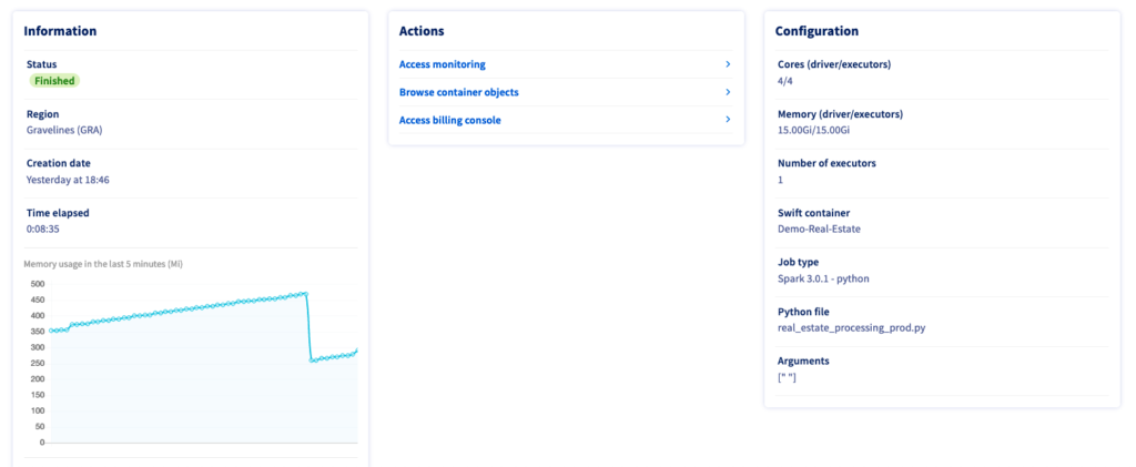
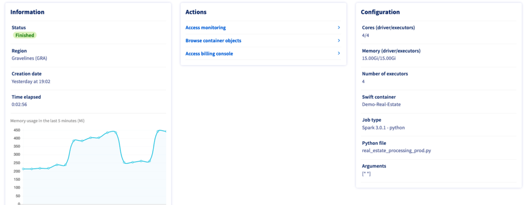
In the first picture, you see the time taken for this job when launching only 1 executor- 8:35 minutes. This duration is reduced to only 2:56 minutes when launching the same job (same code etc…) on 4 executors: almost 3 times faster. And since you pay-as-you go, this will only cost you ~33% more in that case for the same operation done 3 times faster- without any modification to your code, only one argument in the CLI call. Let us now use this data to train a model.

Training the model

To train the model, you are going to use OVHcloud AI notebook to deploy a … notebook! With the following command, you will:

• Deploy a notebook running a Jupyterlab, …
• … pre-configured to run on a VM with 1 GPU, …
• … with several important libraries such as Tensorflow or Pytorch installed, …
• … with your S3 bucket transactions-ecoex-clean synchronized on a high-performance storage cluster that is mounted on /workspace/datain your notebook, …
• … and ready to write the model when it has been trained on the /workspace/model path that will be synchronized with your transactions-ecoex-model when the job is over.

ovhai notebook run one-for-all jupyterlab \
    --name transactions-ecoex-training \
    --framework-version v98-ovh.beta.1 \
    --flavor ai1-1-gpu \
    --gpu 1 \
    --volume transactions-ecoex-clean@GRA/:/workspace/data:RO \
    --volume transactions-ecoex-model@GRA/:/workspace/model:RW

In our case, we launch a notebook with only 1 GPU because the code samples we provide would not leverage several GPUs for a single job. I could adapt my code to parallelize the training phase on multiple GPUs, in which case I could launch a job with up to 4 parallel GPUs.Once this is done, just get the URL of your notebook with the following command and connect to it with your browser:

Once you’re done, just get the URL of your notebook with the following command and connect to it with your browser:

debian@d2-4-gra5:~$ ovhai notebook list
ID                                   STATE   AGE FRAMEWORK   VERSION          EDITOR     URL
525bcb3e-d57b-4111-91ff-4a8759061f75 RUNNING 20m one-for-all v98-ovh.beta.1   jupyterlab https://XXXXXXXXXX.notebook.gra.training.ai.cloud.ovh.net

You can now import the real-estate-training.ipynb file to the notebook with just a few clicks. If you don’t want to import it from the computer you use to access the notebook (for example if like me you use a VM to work and have cloned the git repo on this VM and not on your computer), you can push the .ipynb file to your transactions-ecoex-clean or transactions-ecoex-model bucket and re-synchronize the bucket to your notebook while it runs by using the ovhai notebook pull-data command. You will then find the notebook file in the corresponding directory.

Once you have imported the notebook file to your notebook instance, just open it and follow the directives. If you are interested in the result but don’t want to do it yourself, let’s sum up what the notebook does:

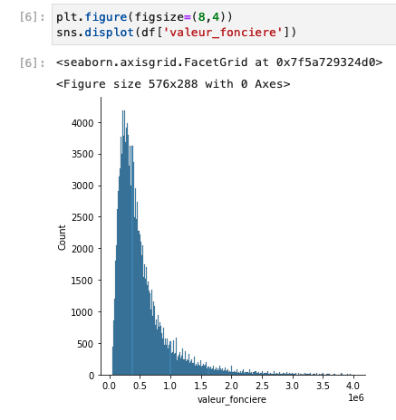
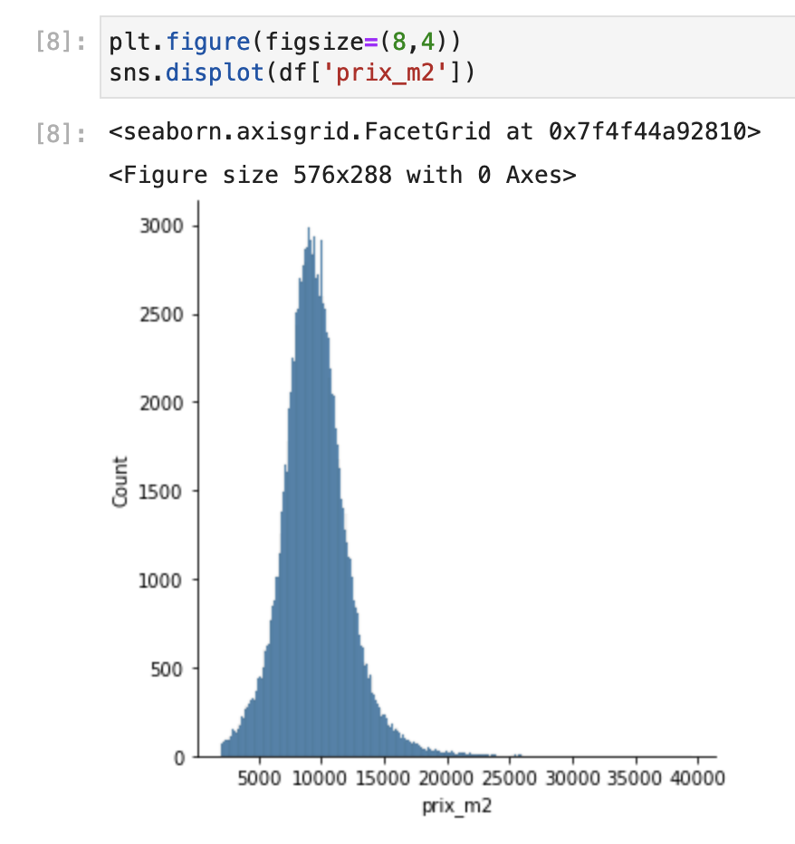
• It reads the clean data from the folder where it has been synchronized from the S3 bucket and plots a few figures.
• In these two plots, you can see that the most represented price range is between 400 and 500k€, and that the price per m² is approximatively a gaussian curve centered on ~10k€. If you know Paris’ real estate market, this shouldn’t surprise you.

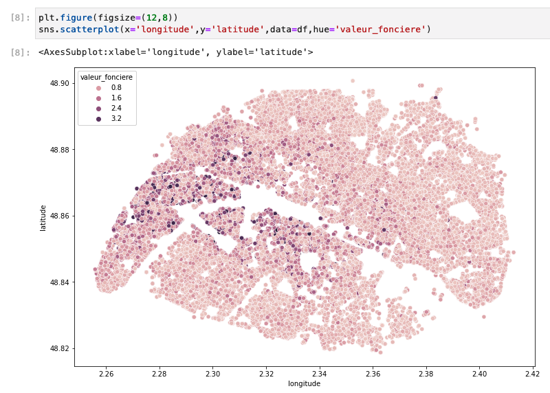
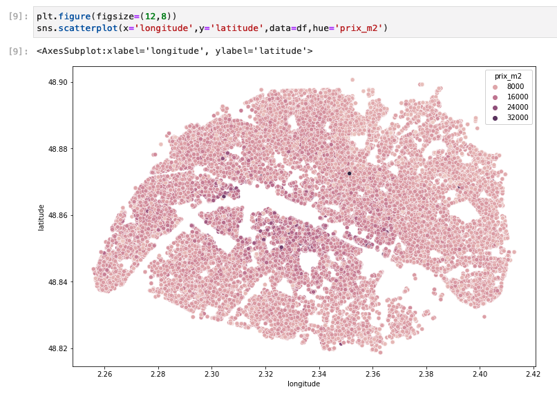
• The next two plots show you the geographical repartition of the prices – absolute and per m². They tell us an interesting story: if you look at the absolute prices, you can see that the West of Paris looks more expensive than the East. However, the price per m² shows that for en equal surface, it is the center of Paris that is more expensive. That means that the center of Paris is relatively more expensive but has smaller flats to offer, so probably less families there!

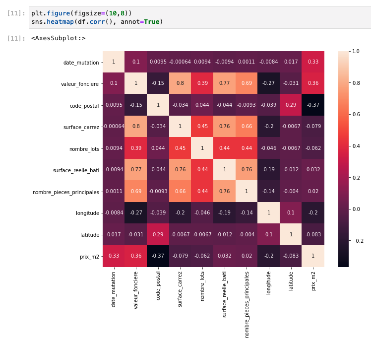
• Finally, a last visualization plot shows you a correlation table of all numerical values contained in the data. Here are a few noteworthy facts:
  • As expected, there is a very high correlation between the absolute price and the surface of a flat. This is common sense for whoever has tried to buy a flat in a city.
  • There is a positive correlation between the price per m² and the date of the transaction: again this is not a surprise as Paris’ real estate steadily increases in value over the years.
  • There is however only a very slightly negative correlation between the surface of a flat and its price per m². This means that the bigger a flat is, the lesser its surface is taken into account in the price. However, this negative correlation is very small so it doesn’t have that much effect.

• After that, the data is transformed a bit to be digestible for the neural network:
  • It is divided in numerical data and categorical data (mainly the street and postal codes);
  • A statistical algorithm is applied to the numerical values to drop outliers that were not dropped in our processing phase by empiric methods;
  • The numerical values are normalized;
  • The categorical data is encoded in discreet numerical values;
  • Finally, the two datasets are merged again.
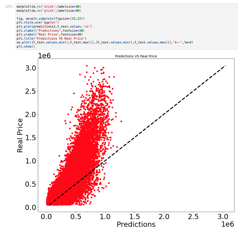
• Once this is done, we create a neural network and finally train a model on a subset of our data! After this first model has been trained, we test it on the remainder of the data. In the next plot, you can see a mapping between the prices predicted by this model and the actual prices. As you can see, our model fares quite poorly and severely undervalues flats most flats.

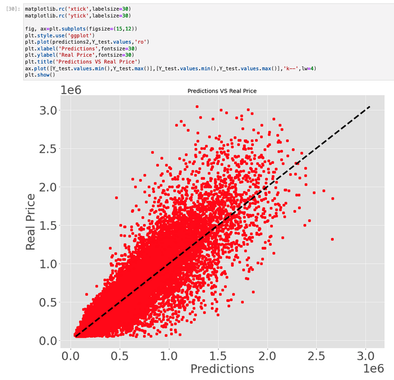
• After this disappointing result, we create a new neural network with more neurons per layer and train it again. The following plot shows its result on our testing set. While it remains quite unprecise and still slightly undervalues flats in average, the results are much better than with the previous model.

• Before stopping the notebook, we save both models to a local directory that will be synchronized to our transactions-ecoex-model S3 bucket.

So, what can we conclude from all of this? First, even if the second model is obviously better than the first, it is still very noisy: while not far from correct on average, there is still a huge variance. Where does this variance come from?

Well, it is not easy to say. To paraphrase the finishing part of my last article:

• We trained this model on only two combinations of basic parameters (the number of neurons per layer). If we were to do that seriously, we would have launched tens or hundreds of trainings in parallel with other parameters and selected the best. There are almost certainly some sets of parameters that would have converged towards a better model.
• Even with the best set of parameters the data is not perfect. How can it differentiate between two flats at the exact same address and with the same surface, one on the ground floor in a narrow street and in front of a very noisy bar, the other on the last floor, higher than the neighbouring buildings, South-oriented towards a calm public garden with a direct view on the Eiffel Tower? The answer is no, as these informations are not contained in the data. And yet, this second flat would probably be more expensive than the first one. Even a very well-trained model would almost certainly overvalue the first one and undervalue the second one.

Conclusion

In this article, I tried to give you a glimpse at the tools that Data Scientists commonly use to manipulate data and train models at scale, in the Cloud or on their own infrastructure:

• Object storage to store the raw and/or clean data;
• Spark or any other distributed processing framework to clean the data – obviously alternatives exist for specific usecase, for example labelling tools to label images when the goal is to train an object detection in images model;
• Notebooks running Machine-Learning frameworks such as Tensorflow, PyTorch, Scikit-Learn etc… to prototype and code algorithms.

Hopefuly, you now have a better understanding on how Machine Learning algorithms work, what their limitations are, and how Data Scientists work on data to create models.

As explained earlier, all the code used to obtain these results can be found here. Please don’t hesitate to replicate what I did or adapt it to other usecases!